Tidy Tuesday Exercise

Author

Joaquin Ramirez

Introduction

This report analyzes the American Idol dataset to explore gender representation among finalists and winners and to investigate any trends or patterns over different seasons. The dataset includes information on eliminations, finalists, seasons, and can be found - Tidy Tuesday Exercise.

Questions: Who is more likely to win the next seasons, a male or a female?

Load Libraries and Data

# Load necessary libraries
library(rlang)

Warning: package 'rlang' was built under R version 4.3.3

library(tidyverse)

Warning: package 'ggplot2' was built under R version 4.3.3

Warning: package 'tidyr' was built under R version 4.3.3

Warning: package 'dplyr' was built under R version 4.3.3

── Attaching core tidyverse packages ──────────────────────── tidyverse 2.0.0 ──
✔ dplyr     1.1.4     ✔ readr     2.1.4
✔ forcats   1.0.0     ✔ stringr   1.5.0
✔ ggplot2   3.5.1     ✔ tibble    3.2.1
✔ lubridate 1.9.2     ✔ tidyr     1.3.1
✔ purrr     1.0.2     
── Conflicts ────────────────────────────────────────── tidyverse_conflicts() ──
✖ purrr::%@%()         masks rlang::%@%()
✖ dplyr::filter()      masks stats::filter()
✖ purrr::flatten()     masks rlang::flatten()
✖ purrr::flatten_chr() masks rlang::flatten_chr()
✖ purrr::flatten_dbl() masks rlang::flatten_dbl()
✖ purrr::flatten_int() masks rlang::flatten_int()
✖ purrr::flatten_lgl() masks rlang::flatten_lgl()
✖ purrr::flatten_raw() masks rlang::flatten_raw()
✖ purrr::invoke()      masks rlang::invoke()
✖ dplyr::lag()         masks stats::lag()
✖ purrr::splice()      masks rlang::splice()
ℹ Use the conflicted package (<http://conflicted.r-lib.org/>) to force all conflicts to become errors

library(here)

Warning: package 'here' was built under R version 4.3.3

here() starts at C:/Users/Joaquin/School/DA - 6833 (Summer 2024)/Joaquin_Ramriez_Portfolio_II

library(janitor)

Warning: package 'janitor' was built under R version 4.3.3


Attaching package: 'janitor'

The following objects are masked from 'package:stats':

    chisq.test, fisher.test

library(gt)
library(tidymodels)

Warning: package 'tidymodels' was built under R version 4.3.3

── Attaching packages ────────────────────────────────────── tidymodels 1.2.0 ──
✔ broom        1.0.5      ✔ rsample      1.2.1 
✔ dials        1.2.1      ✔ tune         1.2.1 
✔ infer        1.0.7      ✔ workflows    1.1.4 
✔ modeldata    1.4.0      ✔ workflowsets 1.1.0 
✔ parsnip      1.2.1      ✔ yardstick    1.3.1 
✔ recipes      1.0.10

Warning: package 'dials' was built under R version 4.3.3

Warning: package 'scales' was built under R version 4.3.3

Warning: package 'infer' was built under R version 4.3.3

Warning: package 'modeldata' was built under R version 4.3.3

Warning: package 'parsnip' was built under R version 4.3.3

Warning: package 'recipes' was built under R version 4.3.3

Warning: package 'rsample' was built under R version 4.3.3

Warning: package 'tune' was built under R version 4.3.3

Warning: package 'workflows' was built under R version 4.3.3

Warning: package 'workflowsets' was built under R version 4.3.3

Warning: package 'yardstick' was built under R version 4.3.3

── Conflicts ───────────────────────────────────────── tidymodels_conflicts() ──
✖ purrr::%@%()         masks rlang::%@%()
✖ scales::discard()    masks purrr::discard()
✖ dplyr::filter()      masks stats::filter()
✖ recipes::fixed()     masks stringr::fixed()
✖ purrr::flatten()     masks rlang::flatten()
✖ purrr::flatten_chr() masks rlang::flatten_chr()
✖ purrr::flatten_dbl() masks rlang::flatten_dbl()
✖ purrr::flatten_int() masks rlang::flatten_int()
✖ purrr::flatten_lgl() masks rlang::flatten_lgl()
✖ purrr::flatten_raw() masks rlang::flatten_raw()
✖ purrr::invoke()      masks rlang::invoke()
✖ dplyr::lag()         masks stats::lag()
✖ yardstick::spec()    masks readr::spec()
✖ purrr::splice()      masks rlang::splice()
✖ recipes::step()      masks stats::step()
• Learn how to get started at https://www.tidymodels.org/start/

library(rsample)  # For data splitting
library(caret)    # For model training

Warning: package 'caret' was built under R version 4.3.3

Loading required package: lattice

Attaching package: 'caret'

The following objects are masked from 'package:yardstick':

    precision, recall, sensitivity, specificity

The following object is masked from 'package:purrr':

    lift

library(glmnet)   # For Ridge and Elastic Net

Warning: package 'glmnet' was built under R version 4.3.3

Loading required package: Matrix

Attaching package: 'Matrix'

The following objects are masked from 'package:tidyr':

    expand, pack, unpack

Loaded glmnet 4.1-8

library(nnet)     # For Neural Network
library(earth)    # For MARS

Warning: package 'earth' was built under R version 4.3.3

Loading required package: Formula
Loading required package: plotmo

Warning: package 'plotmo' was built under R version 4.3.3

Loading required package: plotrix

Warning: package 'plotrix' was built under R version 4.3.2


Attaching package: 'plotrix'

The following object is masked from 'package:scales':

    rescale

library(e1071)    # For SVM


Attaching package: 'e1071'

The following object is masked from 'package:tune':

    tune

The following object is masked from 'package:rsample':

    permutations

The following object is masked from 'package:parsnip':

    tune

library(pROC)     # For evaluation metrics

Warning: package 'pROC' was built under R version 4.3.3

Type 'citation("pROC")' for a citation.

Attaching package: 'pROC'

The following objects are masked from 'package:stats':

    cov, smooth, var

# Define file paths and load data
eliminations <- read_csv(here::here("tidytuesday-exercise", "eliminations.csv"))

Rows: 456 Columns: 46
── Column specification ────────────────────────────────────────────────────────
Delimiter: ","
chr (44): place, gender, contestant, top_36, top_36_2, top_36_3, top_36_4, t...
dbl  (1): season
lgl  (1): comeback

ℹ Use `spec()` to retrieve the full column specification for this data.
ℹ Specify the column types or set `show_col_types = FALSE` to quiet this message.

finalists <- read_csv(here::here("tidytuesday-exercise", "finalists.csv"))

Rows: 190 Columns: 7
── Column specification ────────────────────────────────────────────────────────
Delimiter: ","
chr (6): Contestant, Birthday, Birthplace, Hometown, Description, Contestant...
dbl (1): Season

ℹ Use `spec()` to retrieve the full column specification for this data.
ℹ Specify the column types or set `show_col_types = FALSE` to quiet this message.

seasons <- read_csv(here::here("tidytuesday-exercise", "seasons.csv"))

Rows: 18 Columns: 12
── Column specification ────────────────────────────────────────────────────────
Delimiter: ","
chr (10): winner, runner_up, original_release, original_network, hosted_by, ...
dbl  (2): season, no_of_episodes

ℹ Use `spec()` to retrieve the full column specification for this data.
ℹ Specify the column types or set `show_col_types = FALSE` to quiet this message.

# Clean column names
eliminations <- clean_names(eliminations)
finalists <- clean_names(finalists)
seasons <- clean_names(seasons)

# Display the first few rows and summary of each dataset
head(eliminations)

# A tibble: 6 × 46
  season place gender contestant        top_36 top_36_2 top_36_3 top_36_4 top_32
   <dbl> <chr> <chr>  <chr>             <chr>  <chr>    <chr>    <chr>    <chr> 
1      1 1     Female Kelly Clarkson    <NA>   <NA>     <NA>     <NA>     <NA>  
2      1 2     Male   Justin Guarini    <NA>   <NA>     <NA>     <NA>     <NA>  
3      1 3     Female Nikki McKibbin    <NA>   <NA>     <NA>     <NA>     <NA>  
4      1 4     Female Tamyra Gray       <NA>   <NA>     <NA>     <NA>     <NA>  
5      1 5     Male   R. J. Helton      <NA>   <NA>     <NA>     <NA>     <NA>  
6      1 6     Female Christina Christ… <NA>   <NA>     <NA>     <NA>     <NA>  
# ℹ 37 more variables: top_32_2 <chr>, top_32_3 <chr>, top_32_4 <chr>,
#   top_30 <chr>, top_30_2 <chr>, top_30_3 <chr>, top_25 <chr>, top_25_2 <chr>,
#   top_25_3 <chr>, top_24 <chr>, top_24_2 <chr>, top_24_3 <chr>, top_20 <chr>,
#   top_20_2 <chr>, top_16 <chr>, top_14 <chr>, top_13 <chr>, top_12 <chr>,
#   top_11 <chr>, top_11_2 <chr>, wildcard <chr>, comeback <lgl>, top_10 <chr>,
#   top_9 <chr>, top_9_2 <chr>, top_8 <chr>, top_8_2 <chr>, top_7 <chr>,
#   top_7_2 <chr>, top_6 <chr>, top_6_2 <chr>, top_5 <chr>, top_5_2 <chr>, …

head(finalists)

# A tibble: 6 × 7
  contestant   birthday birthplace hometown description season contestant_gender
  <chr>        <chr>    <chr>      <chr>    <chr>        <dbl> <chr>            
1 Kelly Clark… 24-Apr-… Fort Wort… Burleso… "She perfo…      1 Female           
2 Justin Guar… 28-Oct-… Columbus,… Doylest… "He perfor…      1 Male             
3 Nikki McKib… 28-Sep-… Grand Pra… <NA>     "She had p…      1 Female           
4 Tamyra Gray  26-Jul-… Takoma Pa… Atlanta… "She had a…      1 Female           
5 R. J. Helton 17-May-… Pasadena,… Cumming… "J. Helton…      1 Male             
6 Christina C… 21-Jun-… Brooklyn,… <NA>     ".Christin…      1 Female

head(seasons)

# A tibble: 6 × 12
  season winner     runner_up original_release original_network hosted_by judges
   <dbl> <chr>      <chr>     <chr>            <chr>            <chr>     <chr> 
1      1 Kelly Cla… Justin G… June 11 (2002-0… Fox              Ryan Sea… Paula…
2      2 Ruben Stu… Clay Aik… January 21 (200… Fox              Ryan Sea… Paula…
3      3 Fantasia … Diana De… January 19 (200… Fox              Ryan Sea… Paula…
4      4 Carrie Un… Bo Bice   January 18 (200… Fox              Ryan Sea… Paula…
5      5 Taylor Hi… Katharin… January 17 (200… Fox              Ryan Sea… Paula…
6      6 Jordin Sp… Blake Le… January 16 (200… Fox              Ryan Sea… Paula…
# ℹ 5 more variables: no_of_episodes <dbl>, finals_venue <chr>, mentor <chr>,
#   winner_gender <chr>, runner_up_winner <chr>

# In case these files need to be read.
#songs <- read_csv(here::here("data", "songs.csv"))
#auditions <- read_csv(here::here("data", "auditions.csv"))
#ratings <- read_csv(here::here("data", "ratings.csv"))

Eliminations Analysis

# Calculate gender ratios for eliminations by season
eliminations_gender_ratio <- eliminations %>%
  group_by(season) %>%
  summarize(
    male_eliminations = sum(gender == "Male", na.rm = TRUE),
    female_eliminations = sum(gender == "Female", na.rm = TRUE)
  ) %>%
  mutate(gender_ratio = male_eliminations / (female_eliminations + 1))  # Adding 1 to avoid division by zero

# Display the gender ratio
print(eliminations_gender_ratio)

# A tibble: 18 × 4
   season male_eliminations female_eliminations gender_ratio
    <dbl>             <int>               <int>        <dbl>
 1      1                14                  16        0.824
 2      2                15                  21        0.682
 3      3                12                  20        0.571
 4      4                12                  12        0.923
 5      5                12                  12        0.923
 6      6                12                  12        0.923
 7      7                12                  12        0.923
 8      8                18                  18        0.947
 9      9                12                  12        0.923
10     10                12                  12        0.923
11     11                13                  12        1    
12     12                10                  10        0.909
13     13                10                  10        0.909
14     14                12                  12        0.923
15     15                11                  13        0.786
16     16                12                  12        0.923
17     17                11                   9        1.1  
18     18                 9                  11        0.75

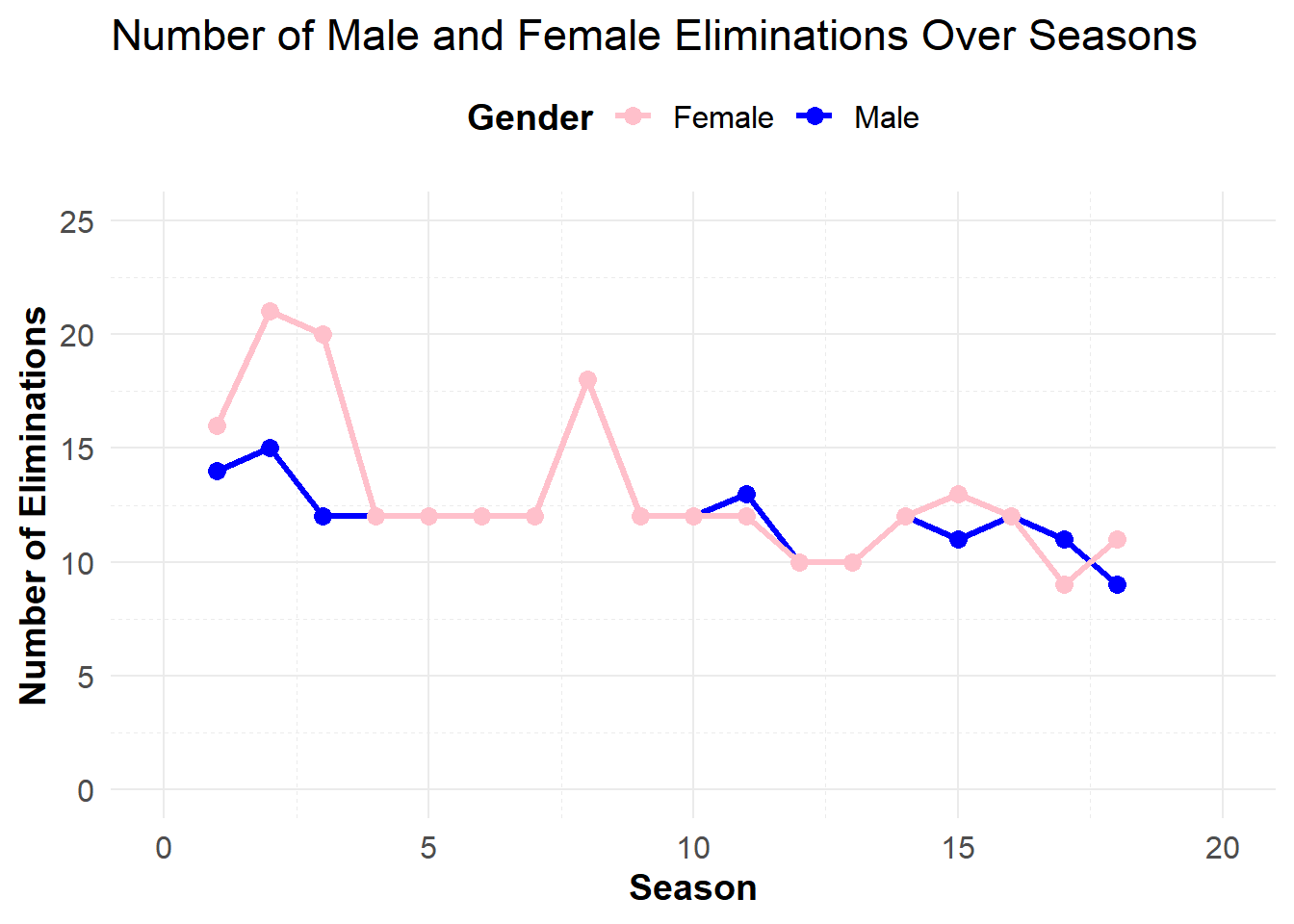
# Plot the number of male and female eliminations over seasons
ggplot(eliminations_gender_ratio, aes(x = season)) +
  geom_line(aes(y = male_eliminations, color = "Male"), size = 1.2) +  # Make lines bolder
  geom_line(aes(y = female_eliminations, color = "Female"), size = 1.2) +  # Make lines bolder
  geom_point(aes(y = male_eliminations, color = "Male"), size = 3) +  # Adjust point size
  geom_point(aes(y = female_eliminations, color = "Female"), size = 3) +  # Adjust point size
  labs(
    title = "Number of Male and Female Eliminations Over Seasons",
    x = "Season",
    y = "Number of Eliminations",
    color = "Gender"  # Customize legend title
  ) +
  scale_color_manual(values = c("Male" = "blue", "Female" = "pink")) +
  scale_x_continuous(limits = c(0, 20)) +  # Set x-axis limits
  scale_y_continuous(limits = c(0, 25)) +  # Set y-axis limits
  theme_minimal(base_size = 14) +  # Use minimal theme with larger base size
  theme(
    legend.position = "top",  # Position the legend at the top
    legend.title = element_text(face = "bold"),  # Bold the legend title
    legend.text = element_text(size = 12),  # Adjust legend text size
    axis.title.x = element_text(face = "bold"),  # Bold x-axis title
    axis.title.y = element_text(face = "bold"),  # Bold y-axis title
    axis.text = element_text(size = 12),  # Adjust axis text size
    panel.grid.major = element_line(size = 0.5, linetype = "solid"),  # Adjust grid line size
    panel.grid.minor = element_line(size = 0.25, linetype = "dashed")  # Adjust grid line size
  )

Warning: Using `size` aesthetic for lines was deprecated in ggplot2 3.4.0.
ℹ Please use `linewidth` instead.

Warning: The `size` argument of `element_line()` is deprecated as of ggplot2 3.4.0.
ℹ Please use the `linewidth` argument instead.

Conclusion:

The elimination data indicates a generally balanced gender ratio across most seasons, with some variability. This suggests that, in terms of eliminations, there is no strong evidence that one gender is systematically favored or disadvantaged.

Winners

# Aggregate the count of male and female winners
winner_counts <- seasons %>%
  group_by(winner_gender) %>%
  summarize(count = n(), .groups = 'drop')

# Print the winner counts to verify
print(winner_counts)

# A tibble: 2 × 2
  winner_gender count
  <chr>         <int>
1 Female            7
2 Male             11

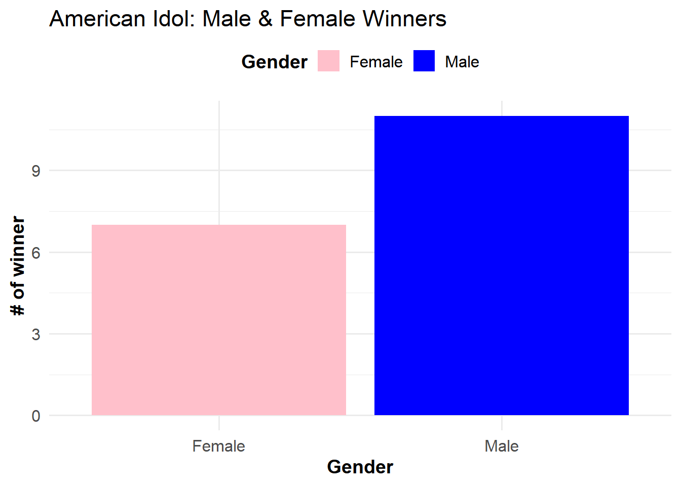
# Create a bar graph of the number of winners by gender
ggplot(winner_counts, aes(x = winner_gender, y = count, fill = winner_gender)) +
  geom_bar(stat = "identity") +
  labs(
    title = "American Idol: Male & Female Winners",
    x = "Gender",
    y = "# of winner",
    fill = "Gender"  # Change legend title to "Gender"
  ) +
  scale_fill_manual(values = c("Male" = "blue", "Female" = "pink")) +
  theme_minimal(base_size = 14) +  # Use minimal theme with larger base size
  theme(
    legend.position = "top",  # Position the legend at the top
    legend.title = element_text(face = "bold"),  # Bold the legend title
    legend.text = element_text(size = 12),  # Adjust legend text size
    axis.title.x = element_text(face = "bold"),  # Bold x-axis title
    axis.title.y = element_text(face = "bold"),  # Bold y-axis title
    axis.text = element_text(size = 12)  # Adjust axis text size
  )

Conclusion:

The American Idol data reveals that out of the 18 seasons analyzed, 7 winners were female and 11 winners were male. This suggests that males have historically been more likely to win the competition compared to females.

Contestants

# Count the number of contestants by season and gender
contestants_by_gender <- finalists %>%
  group_by(season, contestant_gender) %>%
  summarize(count = n(), .groups = 'drop')

# Display the summarized data
print(contestants_by_gender)

# A tibble: 37 × 3
   season contestant_gender count
    <dbl> <chr>             <int>
 1      1 Female                5
 2      1 Male                  5
 3      2 Female                6
 4      2 Male                  6
 5      3 Female                8
 6      3 Male                  4
 7      4 Female                6
 8      4 Male                  6
 9      5 Female                5
10      5 Male                  3
# ℹ 27 more rows

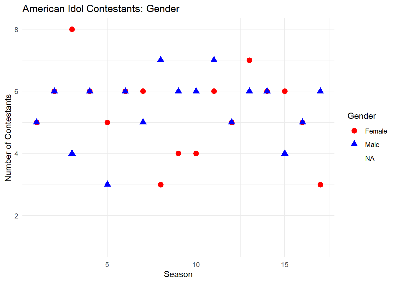
# Create a scatter plot of the number of contestants by gender and season
ggplot(contestants_by_gender, aes(x = season, y = count, color = contestant_gender, shape = contestant_gender)) +
  geom_point(size = 3) +
  labs(title = "American Idol Contestants: Gender",
       x = "Season",
       y = "Number of Contestants",
       color = "Gender",
       shape = "Gender") +
  scale_color_manual(values = c("Male" = "blue", "Female" = "red")) +
  theme_minimal()

Warning: Removed 3 rows containing missing values or values outside the scale range
(`geom_point()`).

Observations:

Across the 17 seasons, there were several seasons with a balanced number of male and female contestants.
Some seasons showed a slight imbalance, such as Season 3 with more females (8) than males (4) and Season 8 with more males (7) than females (3).

Model Fitting

# Load necessary libraries
library(tidymodels)
library(dplyr)

# Prepare data for modeling
seasons_clean <- seasons %>%
  mutate(
    winner_gender = as.factor(winner_gender),
    original_network = as.factor(original_network),
    hosted_by = as.factor(hosted_by),
    judges = as.factor(judges),
    finals_venue = as.factor(finals_venue),
    mentor = as.factor(mentor))

# Split data into training and testing sets
set.seed(123)  # For reproducibility
data_split <- initial_split(seasons_clean, prop = 0.8, strata = winner_gender)
train_data <- training(data_split)
test_data <- testing(data_split)

# Create a recipe for preprocessing
recipe <- recipe(winner_gender ~ season + original_network + hosted_by + judges + no_of_episodes + finals_venue + mentor, data = train_data) %>%
  step_dummy(all_nominal(), -all_outcomes()) %>%  # Convert categorical variables to dummy variables
  step_zv(all_predictors()) %>%  # Remove zero variance predictors
  step_impute_median(all_predictors()) %>%  # Impute missing values
  step_scale(all_predictors()) %>%  # Scale predictors
  step_center(all_predictors())     # Center predictors

# Define model specifications
log_reg_spec <- logistic_reg() %>%
  set_engine("glm")

rf_spec <- rand_forest() %>%
  set_engine("ranger") %>%
  set_mode("classification")

svm_spec <- svm_rbf() %>%
  set_engine("kernlab") %>%
  set_mode("classification")

# Create workflows
log_reg_workflow <- workflow() %>%
  add_recipe(recipe) %>%
  add_model(log_reg_spec)

rf_workflow <- workflow() %>%
  add_recipe(recipe) %>%
  add_model(rf_spec)

svm_workflow <- workflow() %>%
  add_recipe(recipe) %>%
  add_model(svm_spec)

# Fit models with cross-validation
cv_folds <- vfold_cv(train_data, v = 5, strata = winner_gender)

log_reg_fit <- log_reg_workflow %>%
  fit_resamples(cv_folds)

→ A | warning: ! There are new levels in a factor: `NA`.

There were issues with some computations   A: x1

→ B | warning: ! There are new levels in a factor: `NA`., prediction from rank-deficient fit; attr(*, "non-estim") has doubtful cases

There were issues with some computations   A: x1
→ C | warning: glm.fit: fitted probabilities numerically 0 or 1 occurred
There were issues with some computations   A: x1
There were issues with some computations   A: x5   B: x5   C: x2

rf_fit <- rf_workflow %>%
  fit_resamples(cv_folds)

Warning: package 'ranger' was built under R version 4.3.3

→ A | warning: ! There are new levels in a factor: `NA`.
There were issues with some computations   A: x3
There were issues with some computations   A: x10

svm_fit <- svm_workflow %>%
  fit_resamples(cv_folds)

→ A | warning: ! There are new levels in a factor: `NA`.
There were issues with some computations   A: x2
There were issues with some computations   A: x10

# Collect and print metrics
log_reg_metrics <- log_reg_fit %>% collect_metrics()
rf_metrics <- rf_fit %>% collect_metrics()
svm_metrics <- svm_fit %>% collect_metrics()

print(log_reg_metrics)

# A tibble: 3 × 6
  .metric     .estimator  mean     n std_err .config             
  <chr>       <chr>      <dbl> <int>   <dbl> <chr>               
1 accuracy    binary     0.6       5   0.113 Preprocessor1_Model1
2 brier_class binary     0.374     5   0.108 Preprocessor1_Model1
3 roc_auc     binary     0.55      5   0.2   Preprocessor1_Model1

print(rf_metrics)

# A tibble: 3 × 6
  .metric     .estimator  mean     n std_err .config             
  <chr>       <chr>      <dbl> <int>   <dbl> <chr>               
1 accuracy    binary     0.6       5 0.0408  Preprocessor1_Model1
2 brier_class binary     0.229     5 0.00545 Preprocessor1_Model1
3 roc_auc     binary     0.7       5 0.122   Preprocessor1_Model1

print(svm_metrics)

# A tibble: 3 × 6
  .metric     .estimator  mean     n std_err .config             
  <chr>       <chr>      <dbl> <int>   <dbl> <chr>               
1 accuracy    binary     0.533     5  0.122  Preprocessor1_Model1
2 brier_class binary     0.315     5  0.0161 Preprocessor1_Model1
3 roc_auc     binary     0.1       5  0.1    Preprocessor1_Model1

# Select the best model (e.g., Random Forest)
final_rf_model <- rf_workflow %>%
  fit(train_data)

Warning: ! There are new levels in a factor: `NA`.
! There are new levels in a factor: `NA`.

# Predict on the test set
predictions <- predict(final_rf_model, test_data) %>%
  bind_cols(test_data)  # Merge predictions with test_data

Warning: ! There are new levels in a factor: `NA`.

# Rename the prediction column to '.pred_class' for consistency
predictions <- predictions %>%
  rename(.pred_class = .pred_class)

# Evaluate predictions
metrics_test <- metrics(predictions, truth = winner_gender, estimate = .pred_class)
print(metrics_test)

# A tibble: 2 × 3
  .metric  .estimator .estimate
  <chr>    <chr>          <dbl>
1 accuracy binary         0.8  
2 kap      binary         0.545

Conclusion:

Random Forest (RF):

Accuracy: 60% is the same as Logistic Regression, but RF has a lower Brier score (better) and a higher ROC AUC, indicating it has better performance in distinguishing between classes compared to Logistic Regression.
Brier Class Score: The lower score means RF provides better probabilistic predictions than Logistic Regression.
ROC AUC: RF’s higher ROC AUC (0.70) shows better overall performance in class separation.

Logistic Regression (LogReg):

Accuracy: Matches Random Forest, but with a higher Brier score and lower ROC AUC.
Brier Class Score: Higher than RF, indicating less reliable probability estimates.
ROC AUC: Lower than RF, showing poorer performance in distinguishing between classes.

Support Vector Machine (SVM):

Accuracy: Lowest among the models at 53.33%.
Brier Class Score: Higher than RF and LogReg, indicating less reliable probability estimates.
ROC AUC: Very low at 0.10, suggesting that SVM performs poorly in distinguishing between classes.

In other words the best model is the Random Forest which seems to be the most effective model overall, with the highest ROC, AUC and lower Brier score, showing strong performance on the test set with an accuracy of 80% and a moderate Kappa score.

Summary:

This analysis has shown that males have historically been more likely to win American Idol, with Random Forest emerging as the most accurate model for predicting winners based on the available data. The gender ratio among eliminations and finalists does not strongly favor either gender, but the winning trend shows a slight male advantage.

Future Work

Future research could delve into other factors such as judging patterns, audience reactions, and additional contestant characteristics to further understand their impact on the likelihood of winning.