Below is an overview of the key concepts I learned, focusing on predictive modeling techniques and analytics tools with a practical approach using R programming. The topics I explored include:
Data Preprocessing: Techniques for cleaning and transforming raw data to make it suitable for analysis, including handling missing values and normalizing data.
Overfitting and Model Tuning: Understanding the risk of overfitting and employing strategies to optimize model performance through hyperparameter tuning, cross-validation, and regularization methods.
Supervised Methods:
Linear Regression: Analyzing relationships between dependent and independent variables using linear models.
Nonlinear Regression: Addressing more complex relationships between variables with nonlinear models.
Classification: Applying algorithms to classify data into categories, using techniques such as logistic regression, decision trees, and ensemble methods.
Unsupervised Methods:
Clustering: Grouping data into clusters to identify patterns and similarities, utilizing methods such as k-means and hierarchical clustering.
Principal Component Analysis (PCA): Reducing the dimensionality of data to simplify models while preserving essential variability.
Outlier Detection: Identifying and managing outliers to improve model accuracy and robustness.
Advanced Techniques:
Support Vector Machines (SVM): Leveraging SVM for both classification and regression tasks to find optimal decision boundaries and manage high-dimensional data.
Tree-Based Models: Implementing models such as decision trees, Random Forests, and Gradient Boosting to handle complex data structures and improve predictive accuracy.
Through this comprehensive approach, I gained the ability to choose, implement, and interpret predictive models for a variety of applications. I also developed the skills to create detailed and insightful data analysis reports, effectively communicating findings and supporting decision-making processes.
Student Dataset Case Study
R offers a wide range of functions for data preprocessing, calculation, manipulation, and graphical display, and can be easily extended with new functions through downloadable packages from the Comprehensive R Archive Network (CRAN).
As an example, the studentdata dataset from the LearnBayes package is used, containing 657 observations across 11 variables:
Student student number Height height in inches Gender gender Shoes number of pairs of shoes owned Number number chosen between 1 and 10 Dvds name of movie dvds owned ToSleep time the person went to sleep the previous night (hours past midnight) WakeUp time the person woke up the next morning Haircut cost of last haircut including tip Job number of hours working on a job per week Drink usual drink at suppertime among milk, water, and pop
Install LearnBayes package in R/Rstudio and then access studentdata
#Install the LearnBayes package#Keep in mind that R is case-sensitive#install.packages('LearnBayes')#You just need to install once and then you can directly use#so long as you access the LearnBayes packagelibrary(LearnBayes)#Access studentdata from the LearnBayes packagedata(studentdata)attach(studentdata)#show part of datahead(studentdata)
After accessing the studentdata, we can now use R to answer the following questions:
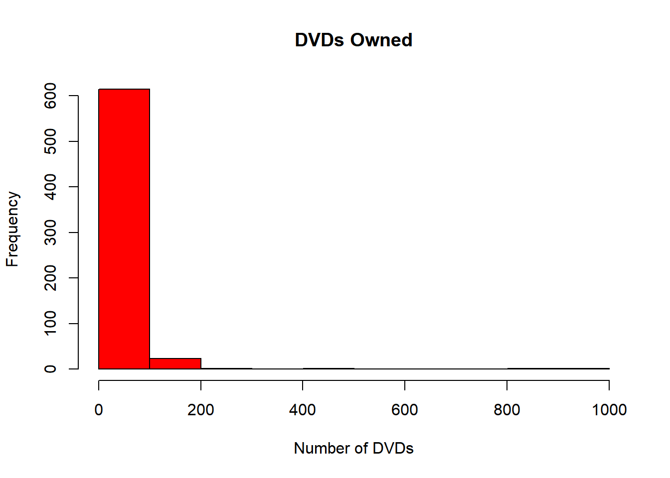
The variable Dvds in the student dataset contains the number of movie DVDs owned by students in the class.
Construct a histogram of this variable using the hist command in R.
#?hist# Construct a histogram of the Dvds variablehist(Dvds,main ="DVDs Owned", xlab ="Number of DVDs", col ="red")
Summarize this variable using the summary command in R.
summary(Dvds)
   Min. 1st Qu.  Median    Mean 3rd Qu.    Max.    NA's
   0.00   10.00   20.00   30.93   30.00 1000.00      16
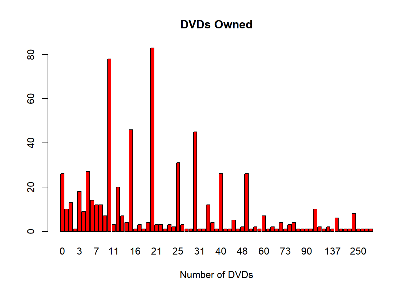
Use the table command in R to construct a frequency table of the individual values of Dvds that were observed. If one constructs a barplot of these tabled values using the command barplot(table(Dvds),col=‘red’) one will see that particular response values are very popular. Is there any explanation for these popular values for the number of DVDs owned?
barplot(table,col='red', main ="DVDs Owned", xlab ="Number of DVDs")
Based on the limited information provided, we can assume there are many reasons for the number of DVDs owned. Some of these reasons include, but are not limited to: sales of DVDs, the release of new or classic DVDs, are students collecting DVDs and DVDs received as gifts. In order to dive deeper into the analysis, it would be crucial to know the name of the movies. This information could provide important details about the reasons why certain DVDs are appearing more often.
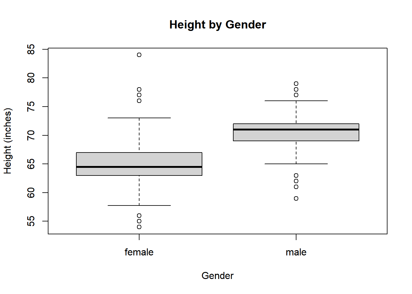
The variable Height contains the height (in inches) of each student in the class.
Construct parallel boxplots of the heights using the Gender variable. Hint: boxplot(Height~Gender)
boxplot(Height~Gender, main ="Height by Gender", ylab ="Height (inches)")
If one assigns the boxplot output to a variable output=boxplot(Height~Gender) then output is a list that contains statistics used in constructing the boxplots. Print output to see the statistics that are stored.
output=boxplot(Height~Gender, main ="Height by Gender", ylab ="Height (inches)")
On average males students are 5.75066 inches taller than female students.
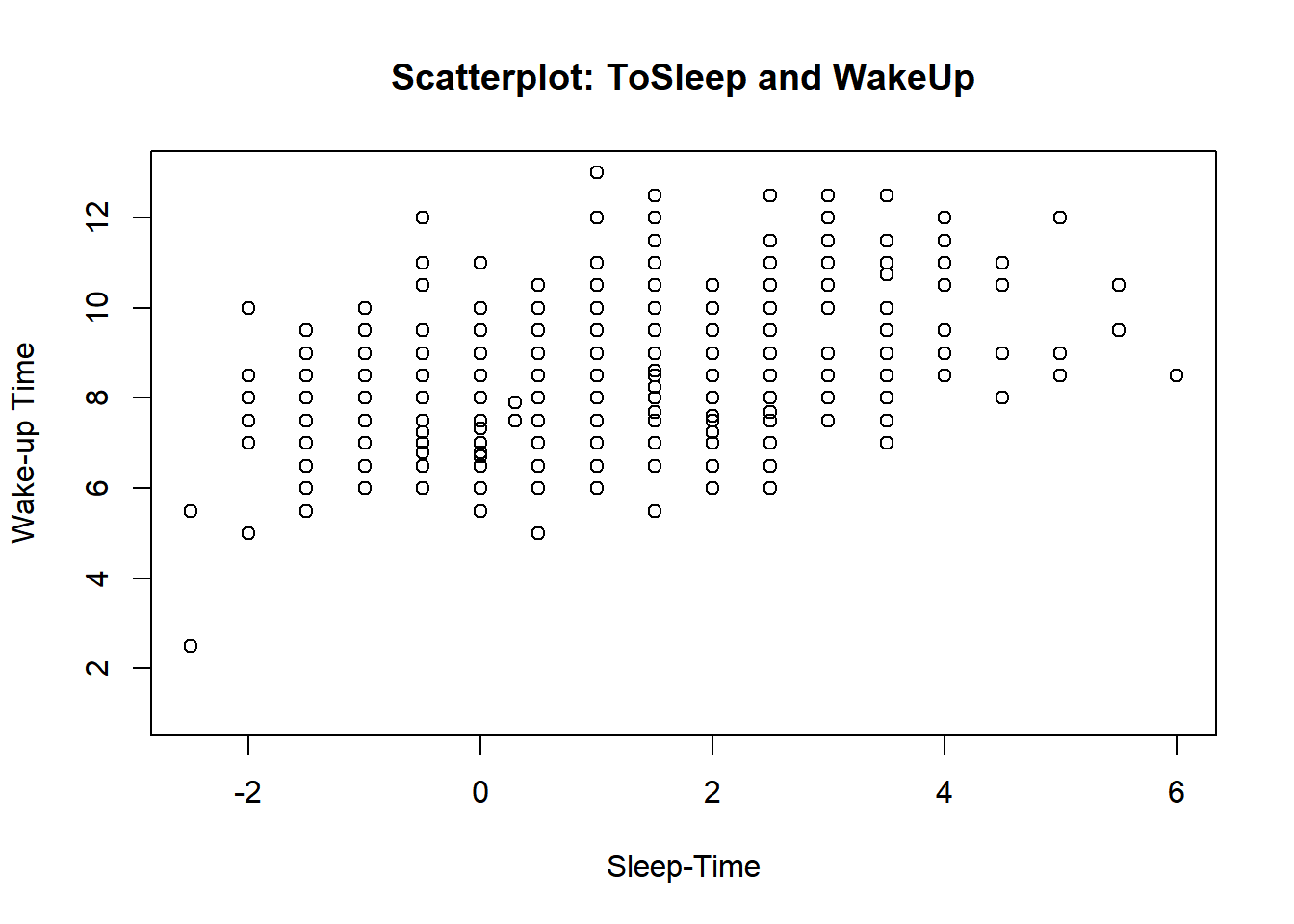
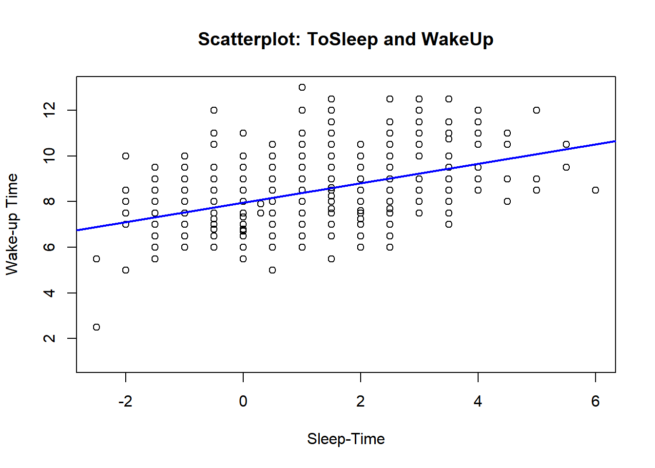
The variables ToSleep and WakeUp contain, respectively, the time to bed and wake-up time for each student the previous evening. (The data are recorded as hours past midnight, so a value of −2 indicates 10 p.m.)
Construct a scatterplot of ToSleep and WakeUp.
plot(ToSleep, WakeUp, main ="Scatterplot: ToSleep and WakeUp", xlab ="Sleep-Time", ylab ="Wake-up Time")
Find a least-squares fit to these data using the lm command and then place the least-squares fit on the scatterplot using the abline command.
plot(ToSleep, WakeUp, main ="Scatterplot: ToSleep and WakeUp", xlab ="Sleep-Time", ylab ="Wake-up Time")fit =lm(WakeUp~ToSleep)summary(fit)
Call:
lm(formula = WakeUp ~ ToSleep)

Residuals:
    Min      1Q  Median      3Q     Max
-4.4010 -0.9628 -0.0998  0.8249  4.6125

Coefficients:
            Estimate Std. Error t value Pr(>|t|)
(Intercept)  7.96276    0.06180  128.85   <2e-16 ***
ToSleep      0.42472    0.03595   11.81   <2e-16 ***
---
Signif. codes:  0 '***' 0.001 '**' 0.01 '*' 0.05 '.' 0.1 ' ' 1

Residual standard error: 1.282 on 651 degrees of freedom
  (4 observations deleted due to missingness)
Multiple R-squared:  0.1765,    Adjusted R-squared:  0.1753
F-statistic: 139.5 on 1 and 651 DF,  p-value: < 2.2e-16
abline(fit, col='blue', lwd=2)
Analysis of Glass Identification Data: Exploratory Data Analysis and Model Development
Warning: package 'mlbench' was built under R version 4.3.3
library(ggplot2)
Warning: package 'ggplot2' was built under R version 4.3.3
Attaching package: 'ggplot2'
The following object is masked from 'package:kernlab':

    alpha
library(GGally)
Warning: package 'GGally' was built under R version 4.3.3
Registered S3 method overwritten by 'GGally':
  method from
  +.gg   ggplot2
library(corrplot)
Warning: package 'corrplot' was built under R version 4.3.3
corrplot 0.92 loaded
library(gridExtra)
Warning: package 'gridExtra' was built under R version 4.3.3
library(AppliedPredictiveModeling)
Warning: package 'AppliedPredictiveModeling' was built under R version 4.3.3
library(caret)
Warning: package 'caret' was built under R version 4.3.3
Loading required package: lattice
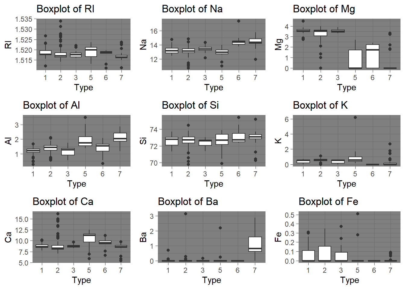
The UC Irvine Machine Learning Repository contains a data set related to glass identification. The data consists of 214 glass samples labeled as one of seven class categories. There are nine predictors, including the refractive index and percentages of eight elements: Na, Mg, Al, Si, K, Ca, Ba, and Fe.
The data can be accessed via
data(Glass)str(Glass)
'data.frame':   214 obs. of  10 variables:
 $ RI  : num  1.52 1.52 1.52 1.52 1.52 ...
 $ Na  : num  13.6 13.9 13.5 13.2 13.3 ...
 $ Mg  : num  4.49 3.6 3.55 3.69 3.62 3.61 3.6 3.61 3.58 3.6 ...
 $ Al  : num  1.1 1.36 1.54 1.29 1.24 1.62 1.14 1.05 1.37 1.36 ...
 $ Si  : num  71.8 72.7 73 72.6 73.1 ...
 $ K   : num  0.06 0.48 0.39 0.57 0.55 0.64 0.58 0.57 0.56 0.57 ...
 $ Ca  : num  8.75 7.83 7.78 8.22 8.07 8.07 8.17 8.24 8.3 8.4 ...
 $ Ba  : num  0 0 0 0 0 0 0 0 0 0 ...
 $ Fe  : num  0 0 0 0 0 0.26 0 0 0 0.11 ...
 $ Type: Factor w/ 6 levels "1","2","3","5",..: 1 1 1 1 1 1 1 1 1 1 ...
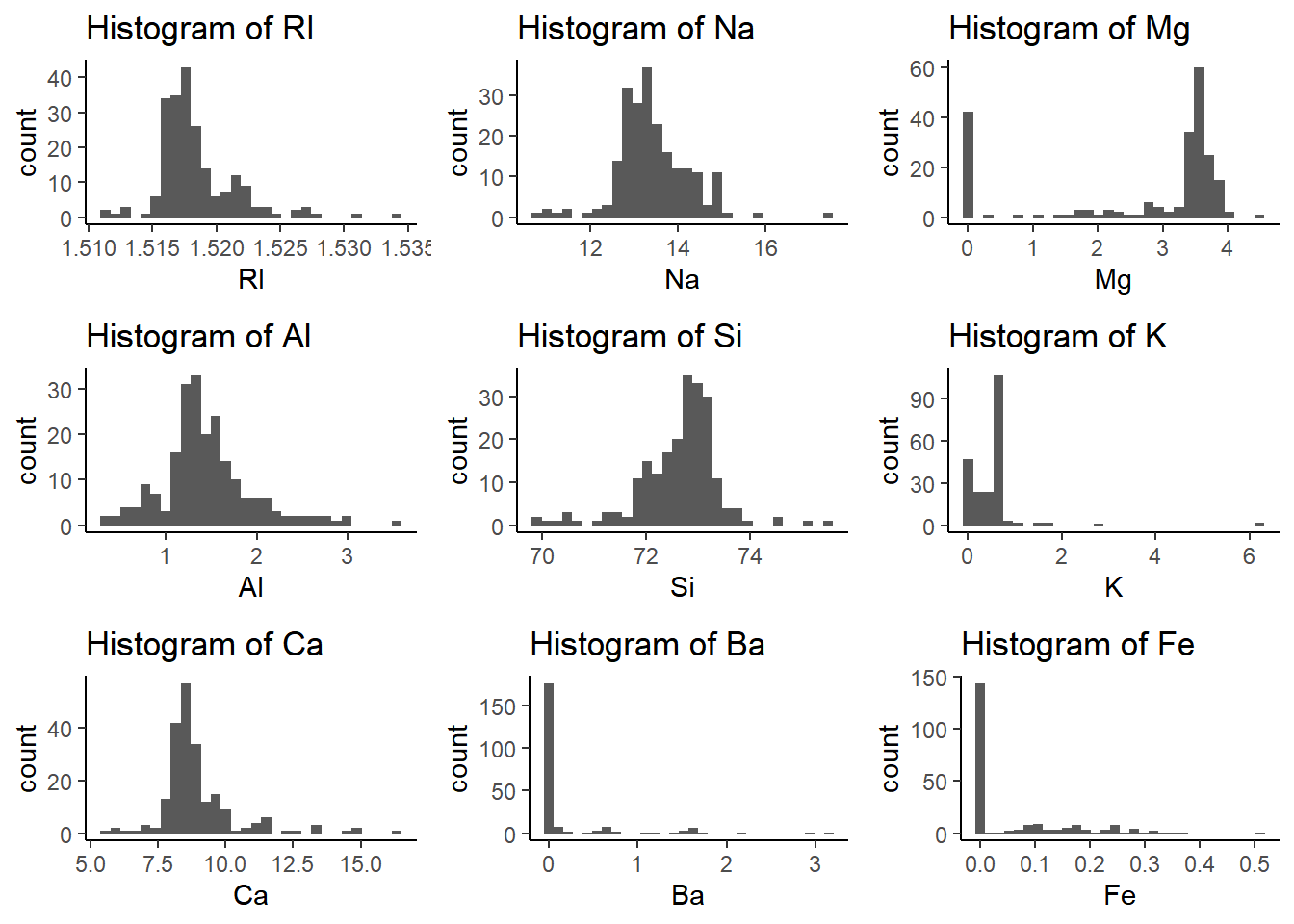
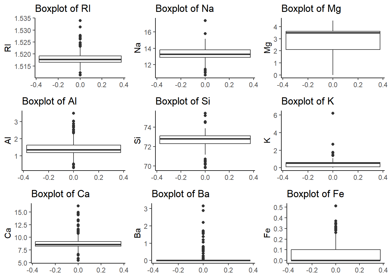
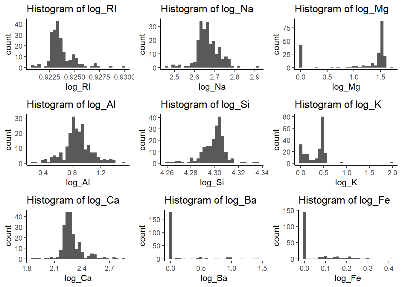
a) Utilize suitable visualizations (employ any types of data visualization you deem appropriate) to explore the predictor variables, aiming to understand their distributions and relationships among them.
Warning: `aes_string()` was deprecated in ggplot2 3.0.0.
ℹ Please use tidy evaluation idioms with `aes()`.
ℹ See also `vignette("ggplot2-in-packages")` for more information.
I utilized both Histograms and Boxplots, you can definitely see a lot of outliers in the plots displayed. Na and Al, seem to be normally distributed but all other seem to be either skewed to the left or to the right.
b) Do there appear to be any outliers in the data? Are any predictors skewed? Show all the work!
We can determine from the observations (Boxplot and Histograms), all but one showed outliers with extreme values. Most of these predictors where either skewed to the left (negative) or to the right (positive). All this to say that we need to consider the outliers and the distribution charactertics going forward.
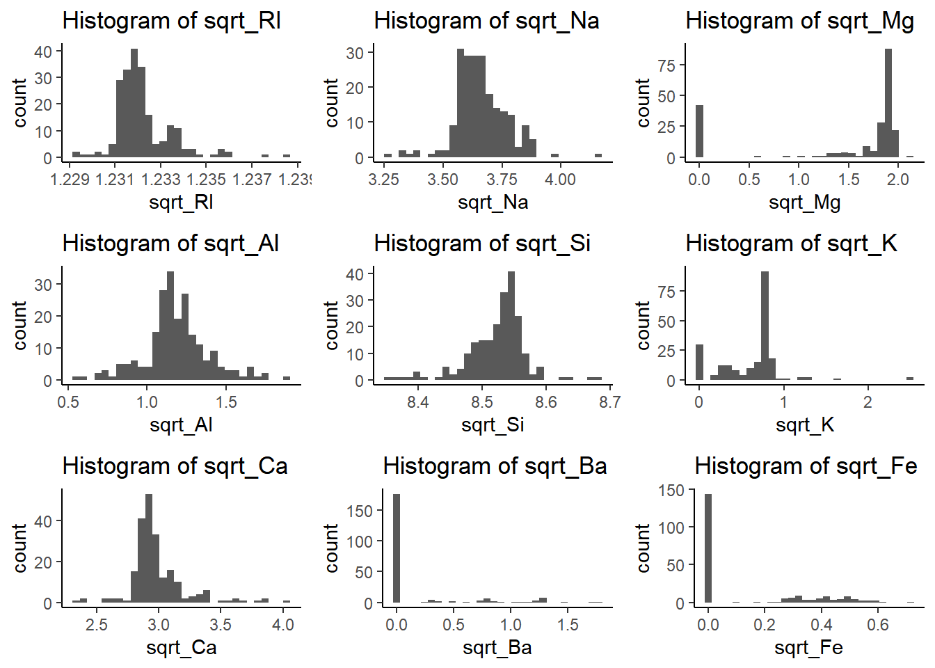
Are there any relevant transformations of one or more predictors that might improve the classification model? Show all the work!
After I applied the transformation and achieved accuracy of 57.5%, and the Kappa is 0.371. We can say there is a level of agreement between the variables. Now looking at the classes that were observed we can see that class 1 and 2 are strong in their classification while the rest need improvement. Maybe if we refine our focus on the variblae we observe we can improve out accurancy.
Fit SVM model (You may refer to Chapter 4 material for details) using the following R codes: (This code will be discussed in detail in the following chapters)
set.seed(231) sigDist <-sigest(Type~ ., data = Glass, frac =1)sigDist
       90%        50%        10%
0.03407935 0.11297847 0.62767315
svmTuneGrid <-data.frame(sigma =as.vector(sigDist)[1], C =2^(-2:10)) svmTuneGrid
set.seed(231)sigDist <-sigest(Type ~ ., data = Glass, frac =1)svmTuneGrid <-data.frame(sigma =as.vector(sigDist)[1], C =2^(-2:10))svmModel <-ksvm(Type ~ ., data = Glass, type ="C-svc", kernel ="rbfdot", kpar =list(sigma =as.vector(sigDist)[1]), C =2^(-2:10))print(svmModel)
Support Vector Machine object of class "ksvm"

SV type: C-svc  (classification)
 parameter : cost C = 0.25
  parameter : cost C = 0.5
  parameter : cost C = 1
  parameter : cost C = 2
  parameter : cost C = 4
  parameter : cost C = 8
  parameter : cost C = 16
  parameter : cost C = 32
  parameter : cost C = 64
  parameter : cost C = 128
  parameter : cost C = 256
  parameter : cost C = 512
  parameter : cost C = 1024

Gaussian Radial Basis kernel function.
 Hyperparameter : sigma =  0.0340793487610772

Number of Support Vectors : 205

Objective Function Value : -30.8971 -8.4786 -4.7642 -3.9839 -4.8778 -8.4545 -6.0399 -4.2908 -6.4624 -4.3643 -3.8975 -4.5021 -3.8506 -4.9211 -4.0869
Training error : 0.439252
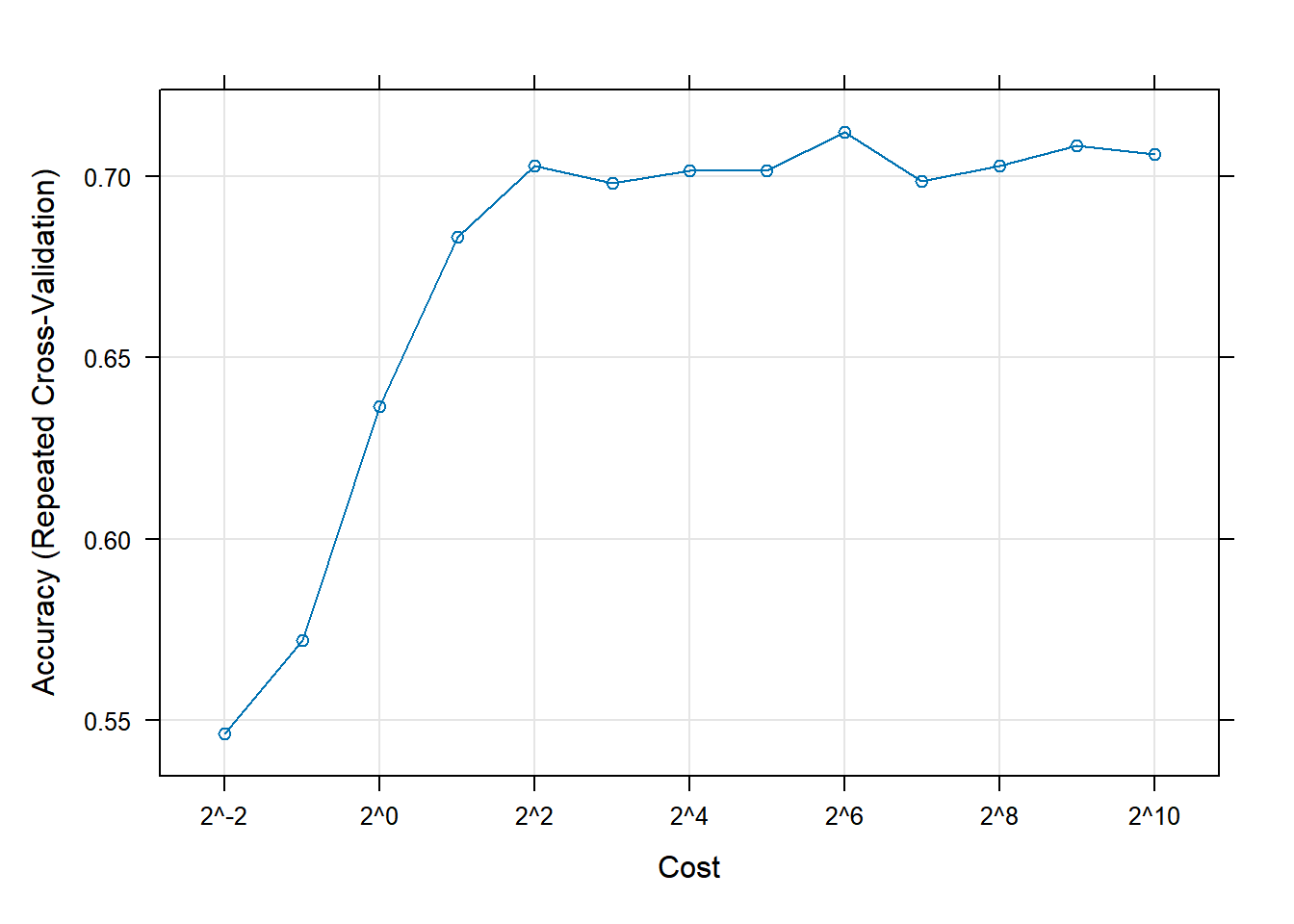
set.seed(1056)# Fit SVM model using 10-fold cross-validationsvmFit <-train(Type ~ .,data = Glass, method ="svmRadial",preProcess =c("center", "scale"),tuneGrid = svmTuneGrid,trControl =trainControl(method ="repeatedcv", repeats =5))plot(svmFit, scales =list(x =list(log =2)))
Predicting Meat Moisture Content Using Infrared Spectroscopy: Model Comparison and Evaluation
Infrared (IR) spectroscopy technology is used to determine the chemical makeup of a substance. The theory of IR spectroscopy holds that unique molecular structures absorb IR frequencies differently. In practice a spectrometer fires a series of IR frequencies into a sample material, and the device measures the absorbance of the sample at each individual frequency. This series of measurements creates a spectrum profile which can then be used to determine the chemical makeup of the sample material.
A Tecator Infratec Food and Feed Analyzer instrument was used to analyze 215 samples of meat across 100 frequencies. A sample of these frequency profiles is displayed in Fig. 6.20. In addition to an IR profile, analytical chemistry determined the percent content of water, fat, and protein for each sample. If we can establish a predictive relationship between IR spectrum and fat content, then food scientists could predict a sample’s fat content with IR instead of using analytical chemistry. This would provide costs savings, since analytical chemistry is a more expensive, time-consuming process
a) Start R and use these commands to load the data:
library(caret)data(tecator)# use ?tecator to see more details?tecator
The matrix absorp contains the 100 absorbance values for the 215 samples, while matrix endpoints contain the percent of moisture, fat, and protein in columns 1–3, respectively. To be more specific
# Assign the percent content to variablesmoisture <- endpoints[,1]fat <- endpoints[,2]protein <- endpoints[,3]
summary(moisture)
   Min. 1st Qu.  Median    Mean 3rd Qu.    Max.
  39.30   55.55   65.70   63.20   71.80   76.60
#print(moisture)
summary(fat)
   Min. 1st Qu.  Median    Mean 3rd Qu.    Max.
   0.90    7.30   14.00   18.14   28.00   49.10
#print(fat)
summary(protein)
   Min. 1st Qu.  Median    Mean 3rd Qu.    Max.
  11.00   15.35   18.70   17.68   20.10   21.80
#print(protein)
# Check for missing valuessum(is.na(absorp))
[1] 0
sum(is.na(moisture))
[1] 0
sum(is.na(fat))
[1] 0
sum(is.na(protein))
[1] 0
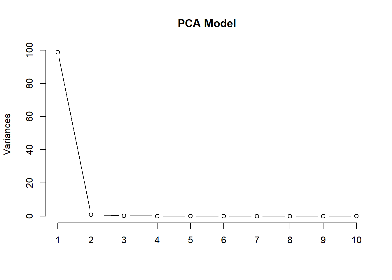
b) In this example the predictors are the measurements at the individual frequencies. Because the frequencies lie in a systematic order (850–1,050nm), the predictors have a high degree of correlation. Hence, the data lie in a smaller dimension than the total number of predictors (215). Use PCA to determine the effective dimension of these data. What is the effective dimension?
# PCA on the absorp datapca_model <-prcomp(absorp, center =TRUE, scale. =TRUE)# Summary of PCA summary(pca_model)
# Scree plot to visualize the variance explained by each componentscreeplot(pca_model, type ="lines", main ="PCA Model")
Based on both the PCA results above, first the pca summary output, and then screeplot visualization, tells me how much of the total variance is explained as PC are added. The following observations come from the output above:
PC1 explains 98.63% of the total variance.
PC2: 0.97% proportion variance, and 99.60% cumulative proportion.
PC3: 0.279% proportion variance, and 99.875% cumulative proportion.
PC4: 0.114% proportion variance, and 99.99% cumulative proportion.
Decision:
As shown in the screeplot and the summary, PC1 explains a very high percentage (98.63%), majority of the variability is captured here. The rest of the pc’s explain additional variance, but they’re unlikely to provide meaningful information.
c) Split the data into a training and a test set the response of the percentage of moisture, pre-process the data, and build at least three models described in this chapter (i.e., ordinary least squares, PCR, PLS, Ridge, and ENET). For those models with tuning parameters, what are the optimal values of the tuning parameter(s)?
Linear Regression

152 samples
  2 predictor

No pre-processing
Resampling: Bootstrapped (25 reps)
Summary of sample sizes: 152, 152, 152, 152, 152, 152, ...
Resampling results:

  RMSE      Rsquared   MAE
  8.521083  0.3199381  6.646874

Tuning parameter 'intercept' was held constant at a value of TRUE
Principal Component Analysis

152 samples
  2 predictor

No pre-processing
Resampling: Cross-Validated (10 fold)
Summary of sample sizes: 136, 136, 137, 138, 136, 138, ...
Resampling results:

  RMSE      Rsquared   MAE
  8.929481  0.2947719  7.356878

Tuning parameter 'ncomp' was held constant at a value of 1
Partial Least Squares

152 samples
  2 predictor

No pre-processing
Resampling: Cross-Validated (10 fold)
Summary of sample sizes: 136, 136, 137, 138, 136, 138, ...
Resampling results:

  RMSE      Rsquared   MAE
  8.918747  0.2967856  7.34553

Tuning parameter 'ncomp' was held constant at a value of 1
Ridge Regression

152 samples
  2 predictor

No pre-processing
Resampling: Cross-Validated (10 fold)
Summary of sample sizes: 136, 136, 137, 138, 136, 138, ...
Resampling results across tuning parameters:

  lambda  RMSE      Rsquared   MAE
  0e+00   8.543739  0.3903416  6.778162
  1e-04   8.543732  0.3903418  6.778158
  1e-01   8.536797  0.3904599  6.774300

RMSE was used to select the optimal model using the smallest value.
The final value used for the model was lambda = 0.1.
glmnet

152 samples
  2 predictor

No pre-processing
Resampling: Cross-Validated (10 fold)
Summary of sample sizes: 136, 136, 137, 138, 136, 138, ...
Resampling results across tuning parameters:

  alpha  lambda      RMSE      Rsquared   MAE
  0.10   0.01016872  8.541750  0.3903215  6.783427
  0.10   0.10168717  8.540506  0.3903110  6.787156
  0.10   1.01687174  8.533382  0.3900054  6.864132
  0.55   0.01016872  8.542255  0.3902511  6.783899
  0.55   0.10168717  8.541134  0.3901088  6.794327
  0.55   1.01687174  8.569440  0.3871371  6.953858
  1.00   0.01016872  8.542709  0.3902184  6.784242
  1.00   0.10168717  8.541940  0.3898954  6.801561
  1.00   1.01687174  8.628888  0.3822190  7.096575

RMSE was used to select the optimal model using the smallest value.
The final values used for the model were alpha = 0.1 and lambda = 1.016872.
Summary:
OLS:
RMSE: 8.521083
Rsquared: 0.3199381
MAE: 6.646874
Tuning parameter held constant at a value of TRUE. (No tuning parameter)
PCR:
RMSE: 8.929481
Rsquared: 0.2947719
MAE: 7.356878
Tuning parameter held constant at a value of 1.
PLS:
RMSE: 8.918747
Rsquared: 0.2967856
MAE: 7.34553
Tuning parameter held constant at a value of 1.
Ridge Regression:
RMSE: 8.536797
Rsquared: 0.3904599
MAE: 6.774300
Tuning parameter the final value used for the model was lambda = 0.1.
Glmnet:
RMSE: 8.541750
Rsquared: 0.3903215
MAE: 6.783427
Tuning parameters alpha = 0.1 and lambda = 0.1016872
Based on the lowest RMSE, OLS and Ridge Regression are the better models. They also they have a high rquared explaining a higher variance proportion.
d) Which model has the best predictive ability? Is any model significantly better or worse than the others?
The models are ordered from best to worst in terms of RMSE (predictive performance), based on the results provided above:
1) OLS:
RMSE: 8.521083
Rsquared: 0.3199381
MAE: 6.646874
Tuning parameter held constant at a value of TRUE. (No tuning parameter)
2) Ridge Regression:
RMSE: 8.536797
Rsquared: 0.3904599
MAE: 6.774300
Tuning parameter the final value used for the model was lambda = 0.1.
3) Glmnet:
RMSE: 8.541750
Rsquared: 0.3903215
MAE: 6.783427
Tuning parameters alpha = 0.1 and lambda = 0.1016872
4) PLS:
RMSE: 8.918747
Rsquared: 0.2967856
MAE: 7.34553
Tuning parameter held constant at a value of 1.
5) PCR:
RMSE: 8.929481
Rsquared: 0.2947719
MAE: 7.356878
Tuning parameter held constant at a value of 1.
The models are ordered first by the lowest RMSE and then highest R-squared to determine their performance. Based on the criteria of lowest RMSE, the OLS model is the best, this tells me that the OLS model has the lowest prediction error. However, you can also get away with using the Ridge model because it has the second lowest RMSE, and highest rsquared, indicating minimal error and a large proportion of the variance is explained by this model.
e) Explain which model you would use for predicting the percentage of moisture of a sample.
The model I would use to predict the percentage of moisture in a sample would be the one with the lowest RMSE because it has the lowest predictive error and a model with a high rsquared which explains variance proportion. In the outputs above, the model that best fits this is the Ridge model.
Comparative Performance of Machine Learning Models on Friedman’s Benchmark Data: Analyzing kNN, MARS, Neural Networks, and SVM
7.2. Friedman (1991) introduced several benchmark data sets create by simulation. One of these simulations used the following nonlinear equation to create data:
where the x values are random variables uniformly distributed between [0, 1] (there are also 5 other non-informative variables also created in the simulation). The package mlbench contains a function called mlbench.friedman1 that simulates these data:
Note: For this exercise, you need to consider at least three of the following models: kNN, MARS, Neural Network, and Support vector machines with a specified kernel.
Warning: package 'earth' was built under R version 4.3.3
Loading required package: Formula
Loading required package: plotmo
Warning: package 'plotmo' was built under R version 4.3.3
Loading required package: plotrix
Warning: package 'plotrix' was built under R version 4.3.2
library(e1071)library(nnet)
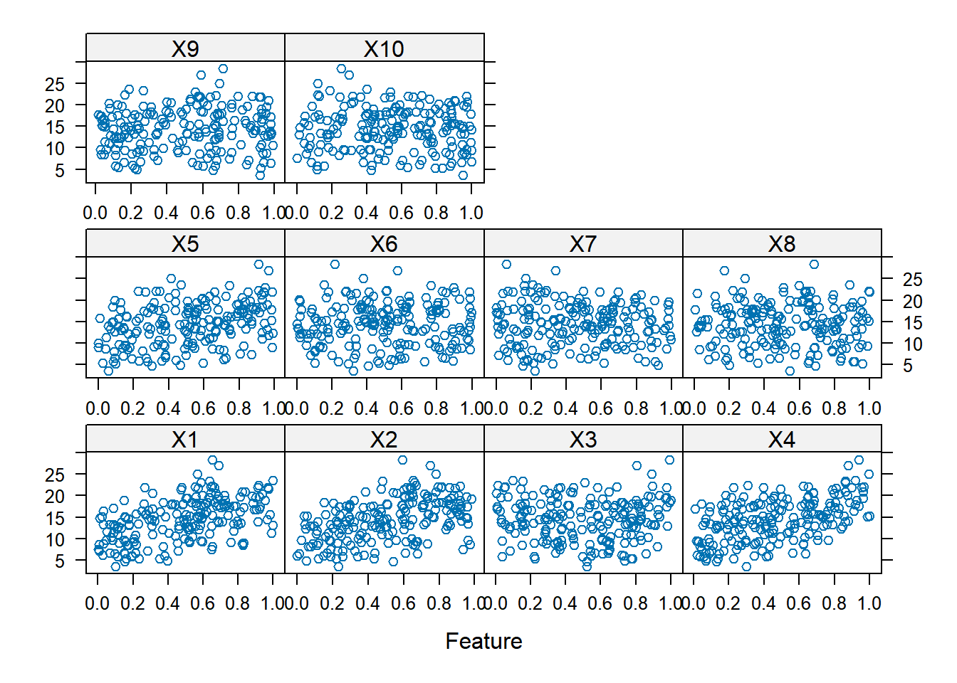
set.seed(200)# Generate training datatrainingData <-mlbench.friedman1(200, sd =1)trainingData$x <-data.frame(trainingData$x) # We convert the 'x' data from a matrix to a data frame. One reason is that this will give the columns names.featurePlot(trainingData$x, trainingData$y) # Visualize the data using featurePlot
# Generate Test DatatestData <-mlbench.friedman1(5000, sd =1) # This creates a list with a vector 'y' and a matrix of predictors 'x'. Also simulate a large test set to estimate the true error rate with good precisiontestData$x <-data.frame(testData$x)
Scatterplot Observations:
X1-X5: show a positive trend.
X6-X10: show no specific trend, no correlation
Tuning several models: kNN, MARS, Neural Network, and SVM.
k-Nearest Neighbors

200 samples
 10 predictor

Pre-processing: centered (10), scaled (10)
Resampling: Bootstrapped (25 reps)
Summary of sample sizes: 200, 200, 200, 200, 200, 200, ...
Resampling results across tuning parameters:

  k   RMSE      Rsquared   MAE
   5  3.466085  0.5121775  2.816838
   7  3.349428  0.5452823  2.727410
   9  3.264276  0.5785990  2.660026
  11  3.214216  0.6024244  2.603767
  13  3.196510  0.6176570  2.591935
  15  3.184173  0.6305506  2.577482
  17  3.183130  0.6425367  2.567787
  19  3.198752  0.6483184  2.592683
  21  3.188993  0.6611428  2.588787
  23  3.200458  0.6638353  2.604529

RMSE was used to select the optimal model using the smallest value.
The final value used for the model was k = 17.
# Predict and evaluate kNN modelknnPred <-predict(knnModel, newdata = testData$x)knnResults <-postResample(pred = knnPred, obs = testData$y) # The function 'postResample' can be used to get the test set perforamnce valuescat("\n\n")
Multivariate Adaptive Regression Spline

200 samples
 10 predictor

Pre-processing: centered (10), scaled (10)
Resampling: Bootstrapped (25 reps)
Summary of sample sizes: 200, 200, 200, 200, 200, 200, ...
Resampling results across tuning parameters:

  nprune  RMSE      Rsquared   MAE
   2      4.383438  0.2405683  3.597961
   3      3.645469  0.4745962  2.930453
   4      2.727602  0.7035031  2.184240
   6      2.331605  0.7835496  1.833420
   7      1.976830  0.8421599  1.562591
   9      1.804342  0.8683110  1.410395
  10      1.787676  0.8711960  1.386944
  12      1.821005  0.8670619  1.419893
  13      1.858688  0.8617344  1.445459
  15      1.871033  0.8607099  1.457618

Tuning parameter 'degree' was held constant at a value of 1
RMSE was used to select the optimal model using the smallest value.
The final values used for the model were nprune = 10 and degree = 1.
Support Vector Machines with Radial Basis Function Kernel

200 samples
 10 predictor

Pre-processing: centered (10), scaled (10)
Resampling: Bootstrapped (25 reps)
Summary of sample sizes: 200, 200, 200, 200, 200, 200, ...
Resampling results across tuning parameters:

  C       RMSE      Rsquared   MAE
    0.25  2.564825  0.7797760  2.011238
    0.50  2.357718  0.7938560  1.837232
    1.00  2.223469  0.8096320  1.723875
    2.00  2.136798  0.8217596  1.659346
    4.00  2.084793  0.8287955  1.622207
    8.00  2.067316  0.8310680  1.611923
   16.00  2.065727  0.8311623  1.610359
   32.00  2.065727  0.8311623  1.610359
   64.00  2.065727  0.8311623  1.610359
  128.00  2.065727  0.8311623  1.610359

Tuning parameter 'sigma' was held constant at a value of 0.062404
RMSE was used to select the optimal model using the smallest value.
The final values used for the model were sigma = 0.062404 and C = 16.
Which models appear to give the best performance? Does MARS select the informative predictors (those named X1–X5)?
Performance Summary:
MARS:
Optimal nprune: 10
RMSE: 1.776575
R-squared: 0.872700
MAE: 1.358367
SVM:
Optimal C: 16
Optimal sigma: 0.068874
RMSE: 2.0889248
R-squared: 0.8232974
MAE: 1.5874122
Neural Network:
Optimal size: 1
Optimal decay: 0.1
RMSE: 2.6493162
R-squared: 0.7177209
MAE: 2.0295251
kNN:
Optimal k: 19
RMSE: 3.2286834
R-squared: 0.6871735
MAE: 2.5939727
I have order the models from best performance to least, based on the following metric, low RMSE, high rsquared, and low MAE. In conclusion the MARS model outperforms the other models, it displays lowest RMSE, highest rsquared, lowest MAE. Now, the SVM model is also a strong contender following after the MARS model, it performs well. The Nueral Network performs alright it does have much higher RMSE than the previous two, lower rsquared and higher MAE, while the kNN model unperformed.
# Variable Importance for MARS Modelcat("Variable for MARS Model:\n")
Positive Scores: V1, V2, V4, and V5 have positive scores. These are categorized as important predictors.
Negative Scores: V6, V7, V8, V9, and V10 have negative scores. These are categorized as counterproductive predictions.
V1 has the highest score (8.732) it is the most influential predictor in the model.
Did the random forest model significantly use the uninformative predictors (V6 – V10)?
No, the variables of importance score for these predictors are either low or negative. As stated above these predictors are categorized as counterproductive, so the models performance is driven by the important predictors.
(b) Now add an additional predictor that is highly correlated with one of the informative predictors. For example:
Fit another random forest model to these data. Did the importance score for V1 change? What happens when you add another predictor that is also highly correlated with V1?
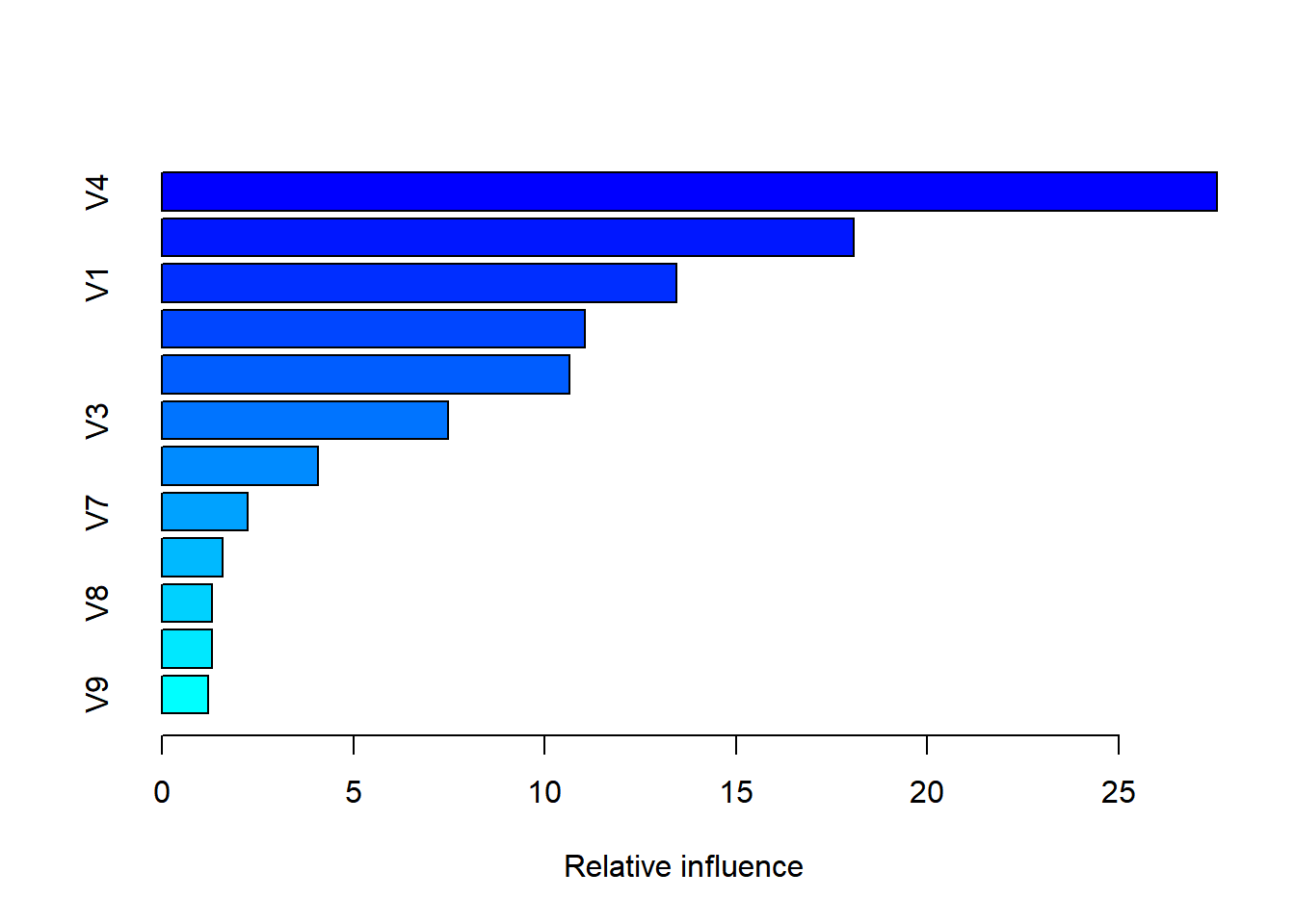
After adding another predictor V1 decreased to 5.60.
V1 and V2, ad V4 have the highest scores.
Duplicate1, has a score of 4.24.
Duplicate2, had a score of 2.45.
V4 has the highest score (7.28) it is the most influential predictor in the model.
As we add more predictors that are highly correlated, it ends up balancing the distribution of the predictor and shifting the level of importance for the model.
(c) Use the cforest function in the party package to fit a random forest model using conditional inference trees. The party package function varimp can calculate predictor importance. The conditional argument of that function toggles between the traditional importance measure and the modified version. Do these importances show the same pattern as the traditional random forest model?
library(party)
Warning: package 'party' was built under R version 4.3.3
Loading required package: grid
Loading required package: mvtnorm
Loading required package: modeltools
Loading required package: stats4
Attaching package: 'modeltools'
The following object is masked from 'package:kernlab':

    prior
Loading required package: strucchange
Warning: package 'strucchange' was built under R version 4.3.3
Loading required package: zoo
Attaching package: 'zoo'
The following objects are masked from 'package:base':

    as.Date, as.Date.numeric
Loading required package: sandwich
Warning: package 'sandwich' was built under R version 4.3.3
In summary, while the general pattern of importance is similar, where V4 has the highest score followed by V2. Additionally, V6 through V10 remain unimportant. The conditional model has a more balance dispenserment while the traditional highlights more the importance of some variables.
(d) Repeat this process with different tree models, such as boosted trees and Cubist. Does the same pattern occur?
Boosted Trees
library(gbm)
Warning: package 'gbm' was built under R version 4.3.3
Loaded gbm 2.2.2
This version of gbm is no longer under development. Consider transitioning to gbm3, https://github.com/gbm-developers/gbm3
set.seed(200)gbm_model <-gbm(y ~ ., data = simulated, distribution ="gaussian", n.trees =1000, interaction.depth =3)summary(gbm_model)
In short the Boosted Model, still considers the level of importance from V6-V10 to be unimportant. The most important variable here is V4 which matches the previous models, followed by V2 and V1. This seem to be in alignment with the other approaches where the level of importance lies within either V4, V1 or V2.
Cubist Model
library(Cubist)
Warning: package 'Cubist' was built under R version 4.3.3
           Length Class      Mode
importance 1      data.frame list
model      1      -none-     character
calledFrom 1      -none-     character
As for the Cubist Model, you have some similarities, where V7-V10 remain unimportant and gives a slightly higher score to V6. However, in comparison to the other scores, V2 has the highest score followed by V1 then V4. This also aligns with the other methods where the level of importance is given to the op three variables either V1, V2, or V4.
Overall the pattern remains almost unchanged you have the order of importance shift between variables, but most of the attention lies within V1, V2, V4. The counterproductive variables are pretty much the same besides in the last model, where it give V6 a higher score, but the pattern remains unchanges for the most part.
[Exploring Predictive Modeling and Data Analysis: An Investigation into Housing Data, Soybean Disease Prediction, Oil Classification, and Statistical Concepts]
library(MASS)
This exercise involves the Boston housing data set.
a) To begin, load in the Boston data set. Since the Boston data set is part of the MASS library, you need to install the MASS package into R/Rstudio and then access the package as follows:
#Boston?Boston #Read about the data set using
How many rows are in this Boston data set? How many columns? What do the rows and columns represent?
data("Boston")
Based on the information provided we have the following:
Rows:506-observations in the dataset for the Boston area.
Columns: 14-variables, each column represents different variables. They are as followed:
crim: per capita crime rate by town.
zn: proportion of residential land zoned for lots over 25,000 sq. ft.
indus: proportion of non-retail business acres per town.
chas: Charles River dummy variable (1 if tract bounds river; 0 otherwise).
nox: nitrogen oxides concentration (parts per 10 million).
rm: average number of rooms per dwelling.
age: proportion of owner-occupied units built prior to 1940.
dis: weighted mean of distances to five Boston employment centers.
rad: index of accessibility to radial highways.
tax: full-value property tax rate per $10,000.
ptratio: pupil-teacher ratio by town.
black: 1000(Bk - 0.63)^2 where Bk is the proportion of blacks by town.
lstat: percentage of lower status of the population.
medv: median value of owner-occupied homes in $1000s.
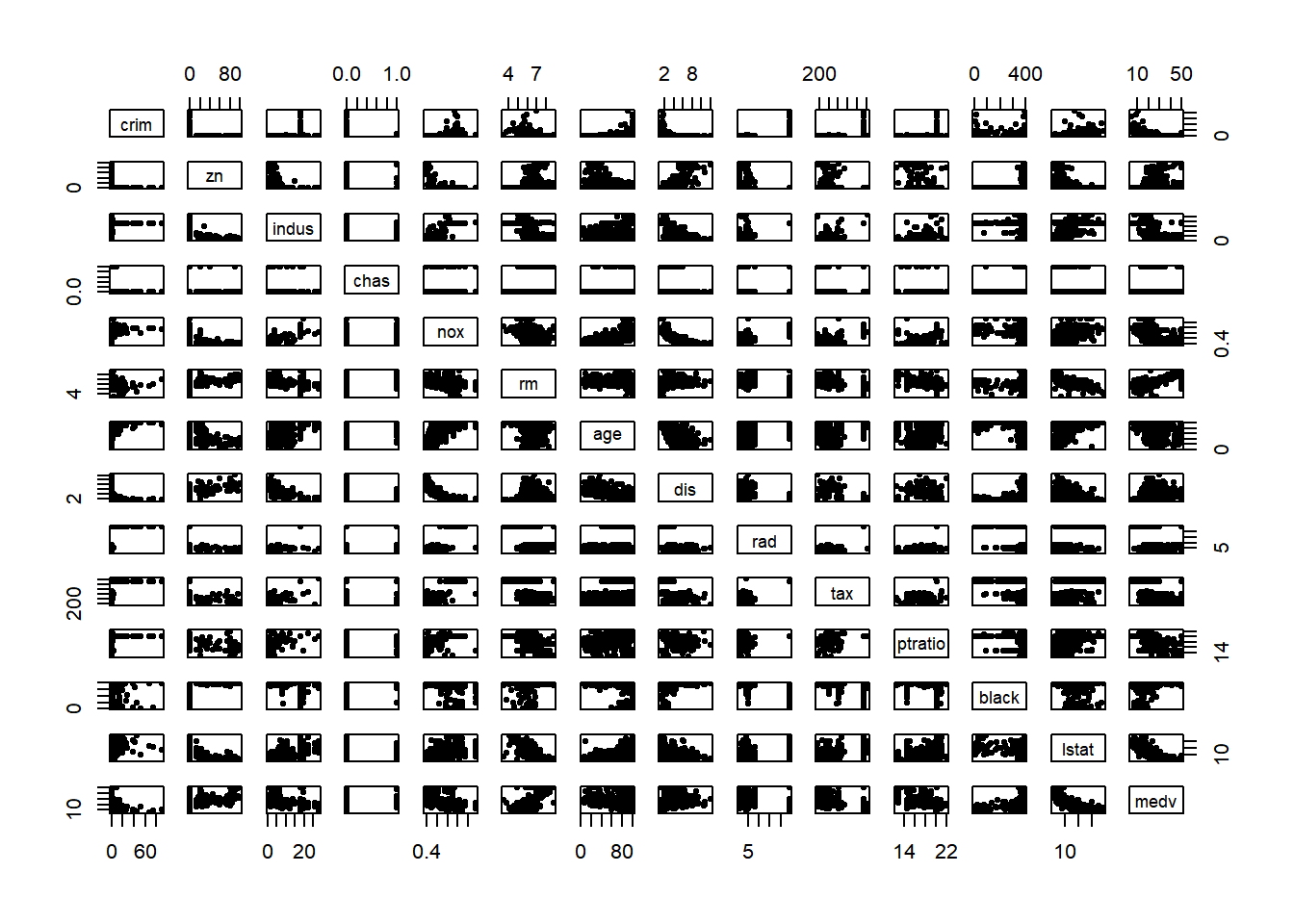
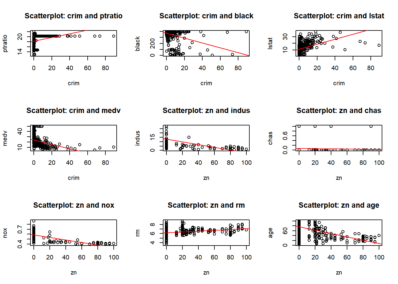
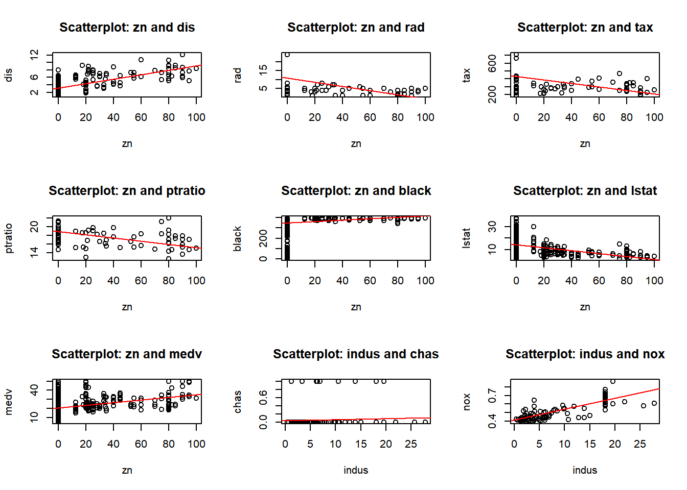
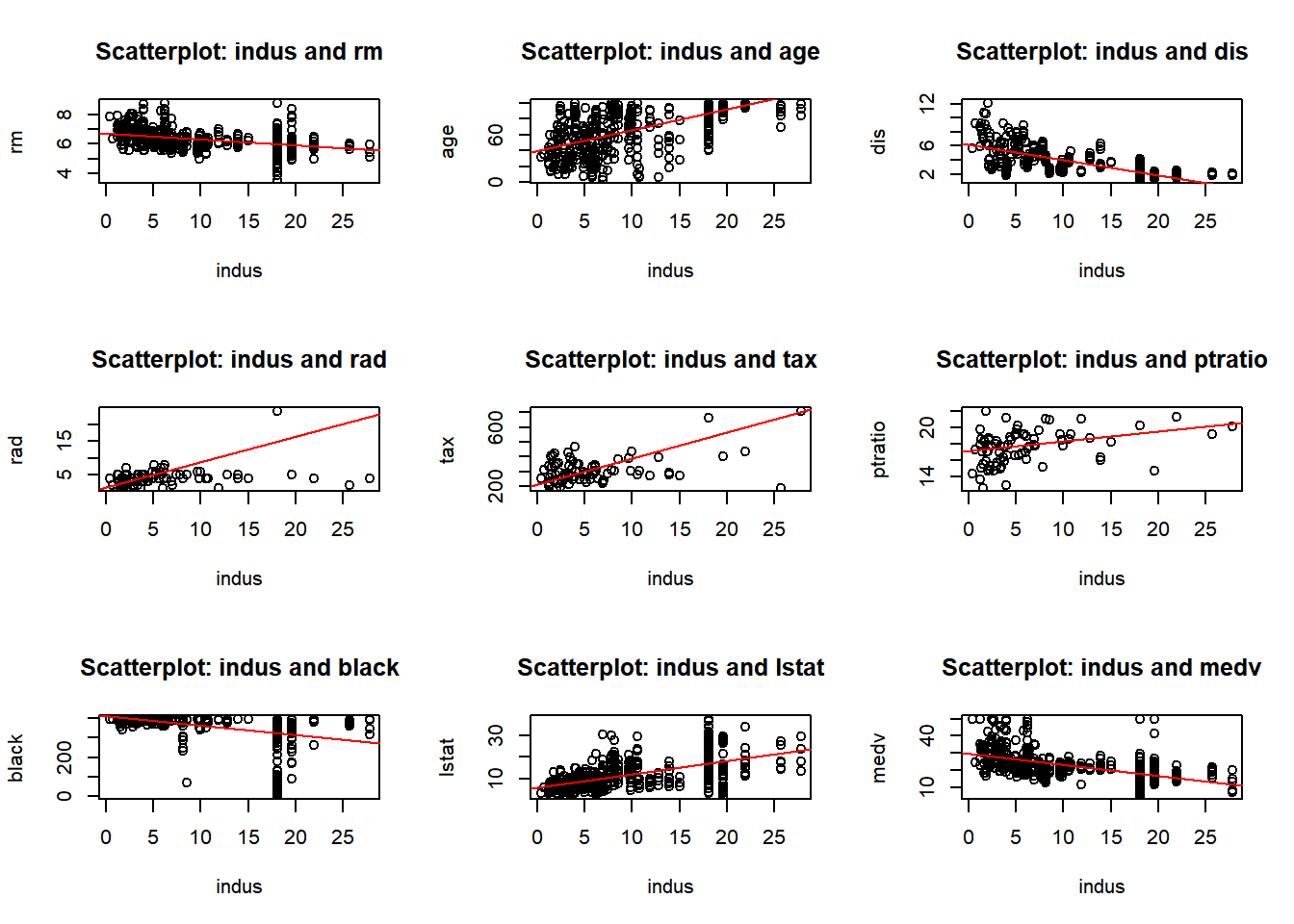
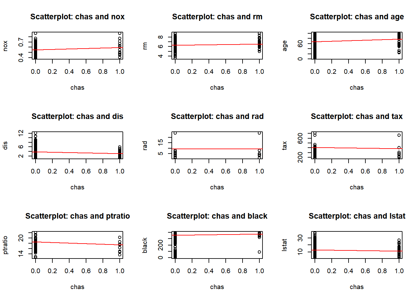
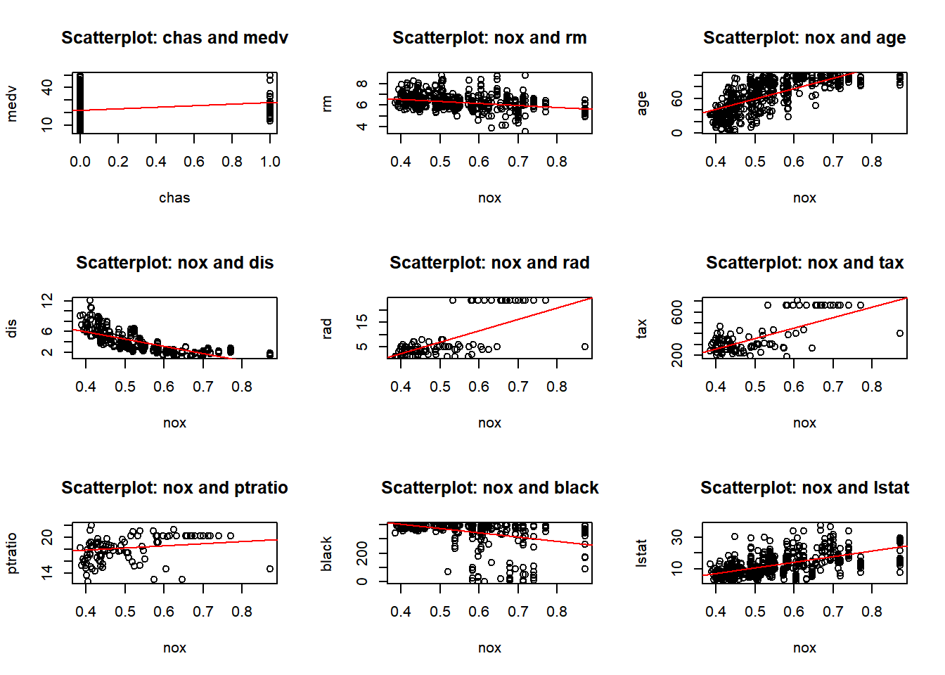
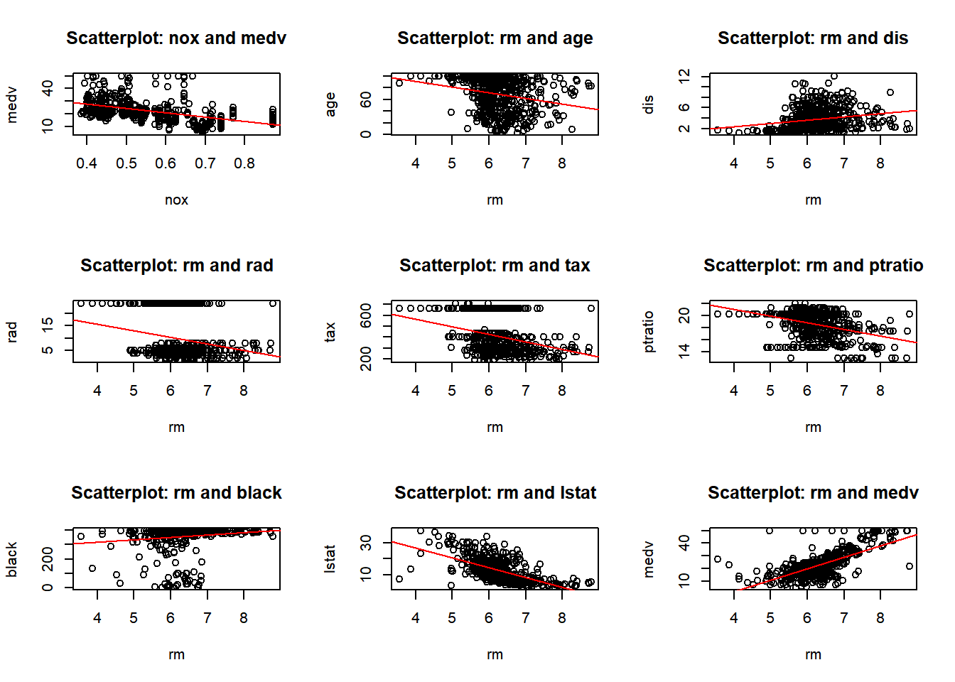
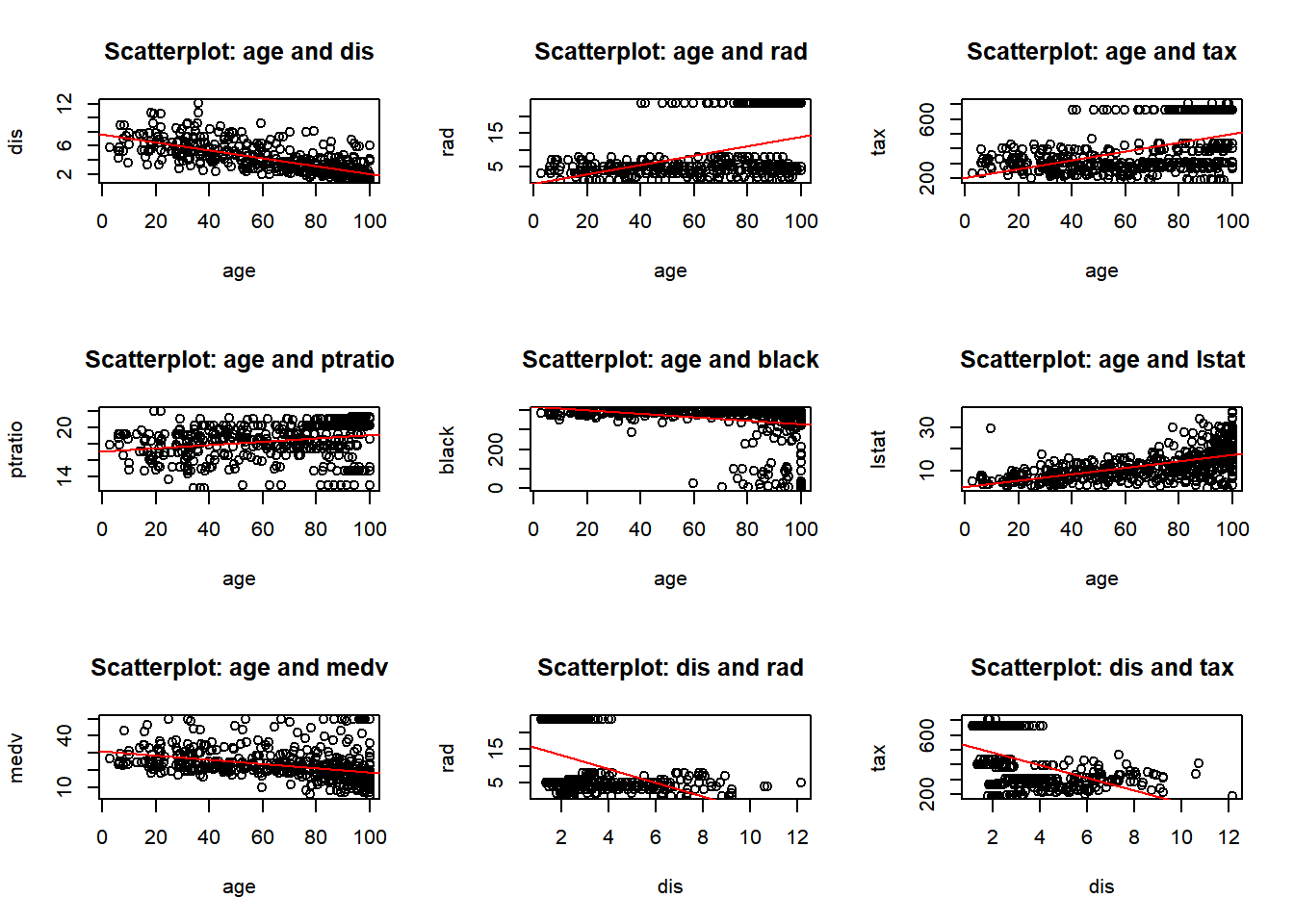
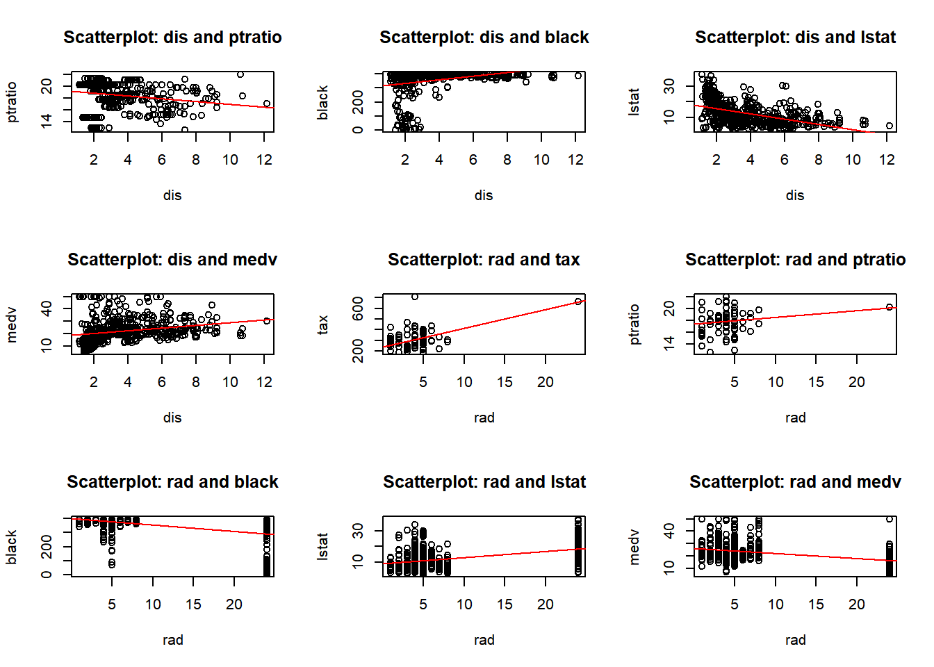
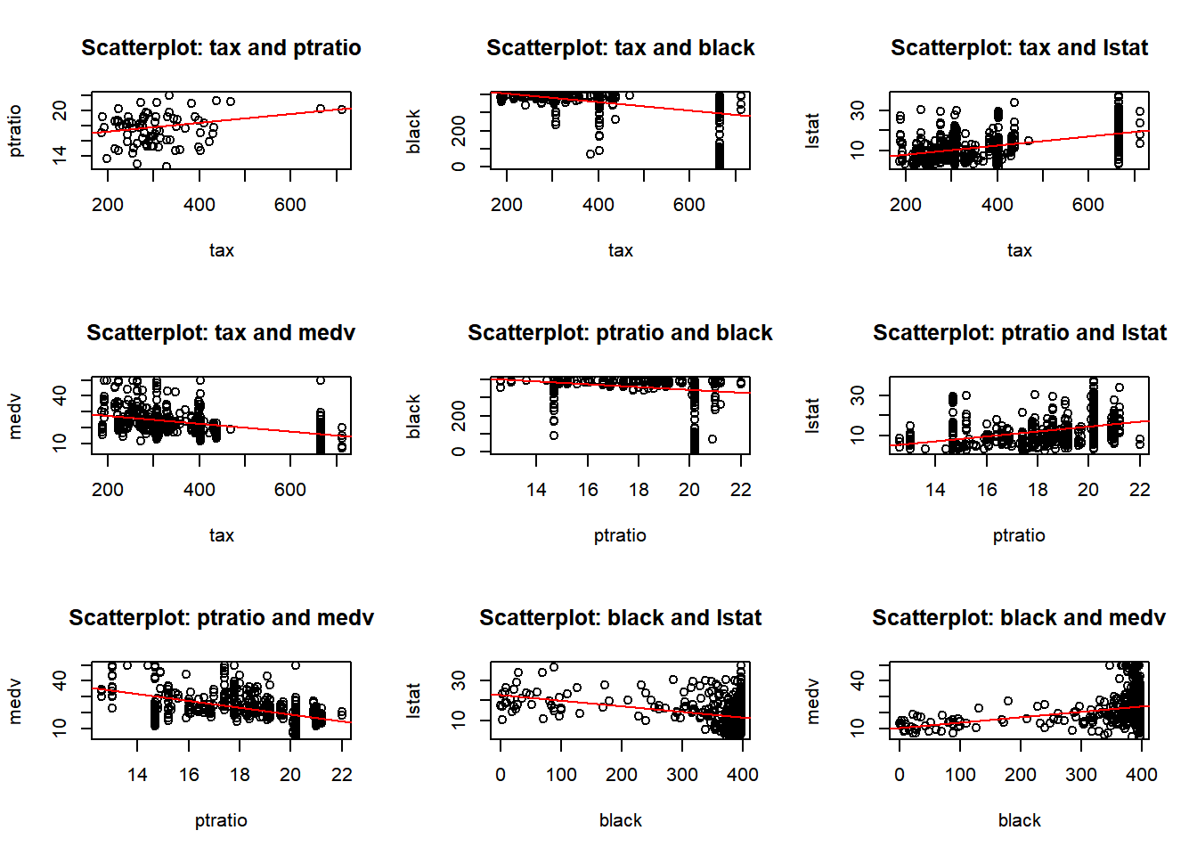
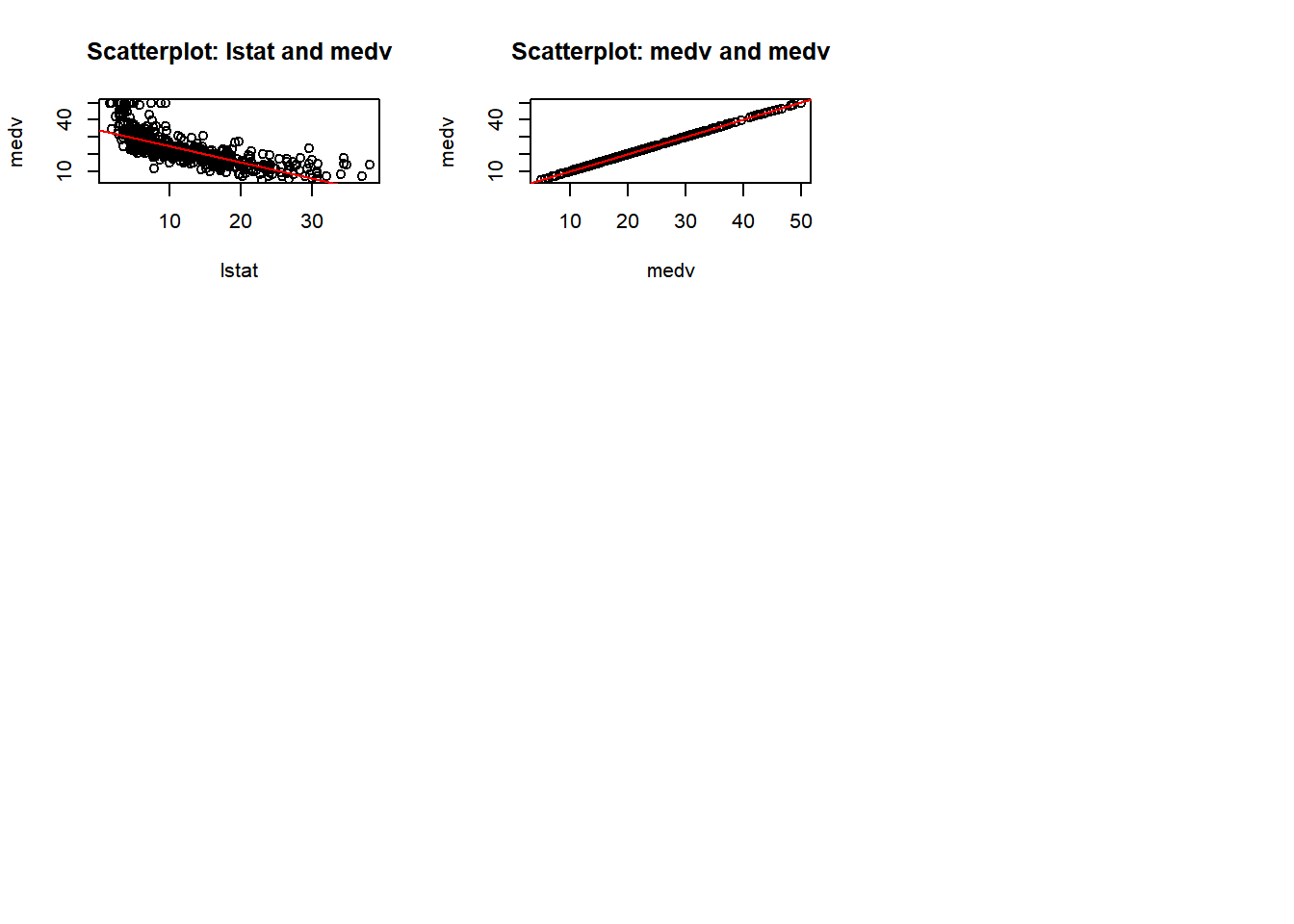
b) Make some pairwise scatterplots of the predictors (columns) in this data set. Describe your findings.
predictors <-colnames(Boston)par(mfrow =c(3, 3)) for (i in1:length(predictors)) {for (j in (i+1):length(predictors)) {predictor_x <- predictors[i] predictor_y <- predictors[j]if (!is.na(predictor_x) &&!is.na(predictor_y)) {plot(Boston[[predictor_x]], Boston[[predictor_y]],xlab = predictor_x, ylab = predictor_y,main =paste("Scatterplot:", predictor_x, "and", predictor_y))abline(lm(Boston[[predictor_y]] ~ Boston[[predictor_x]]), col ="red")}}}
I have provided two displays. The first combines all pairwise plots in a single view, the second organizes them for a better visualization. After reviewing the pairwise plots, I observed both positive and negative correlations, as well as some no-correlation, and some outliers. Below are a few observations, and as I proceed with the homework I will call out other observations:
rad and zn: Negative correlation. Areas in Boston with more accessible radial highways have less residential zoning.
age and lstat: Positive correlation. Older homes have higher proportions of lower status population.
nox and tax: Positive correlation. Higher nitrogen oxides concentration levels are found in areas with higher property taxes.
chas: No significant correlation. Most of the variables associated (chas) - proximity to the Charles River are not significantly.
indus and tax: Positive correlation. Industrialized areas tend to have higher property taxes.
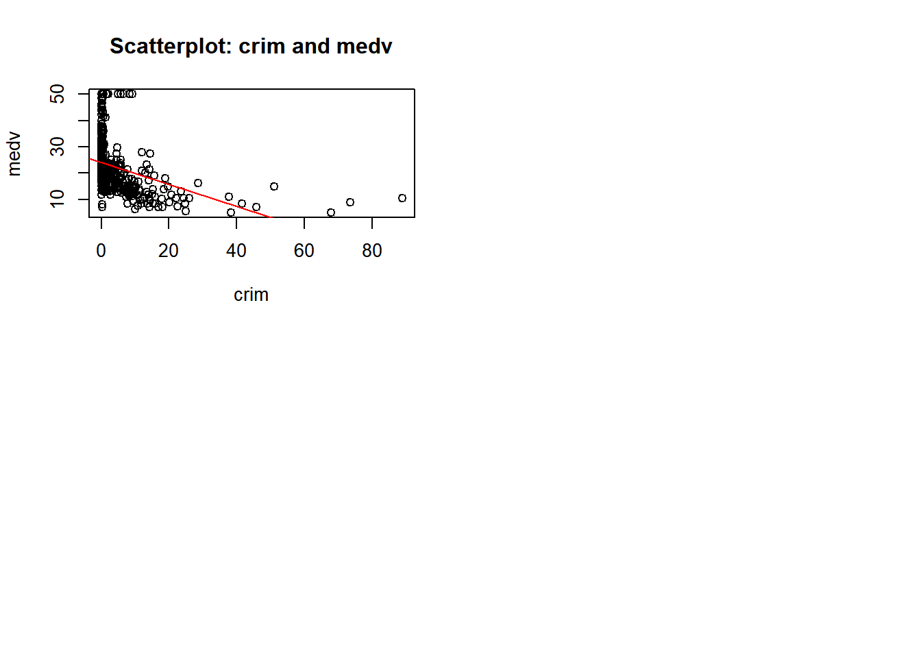
crim and medv: Negative correlation. Higher crime rates are found in areas with median home values.
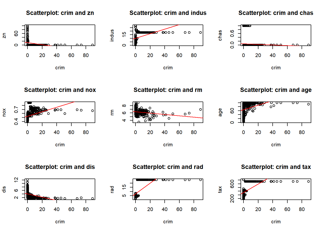
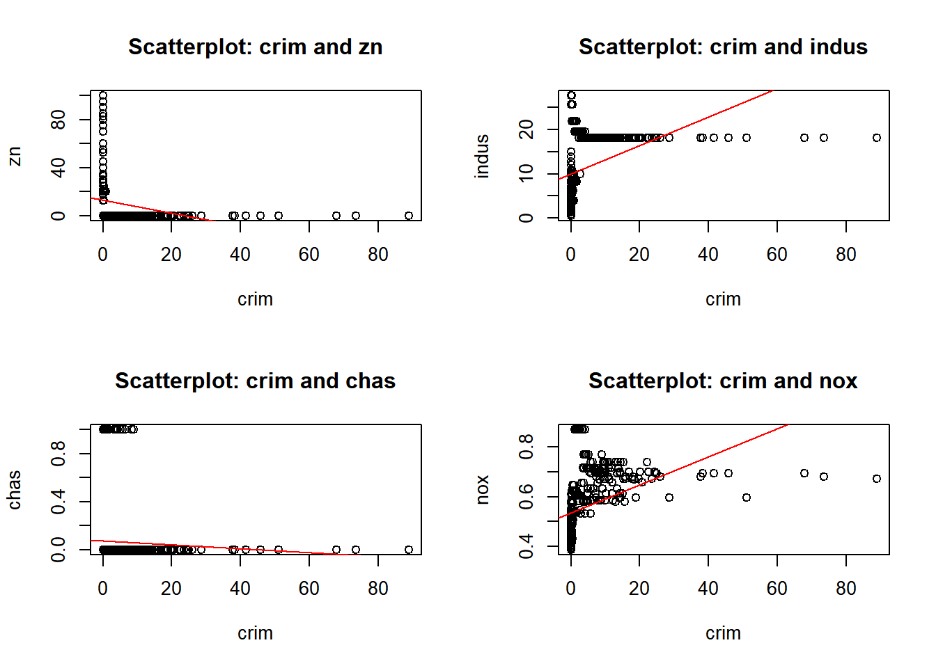
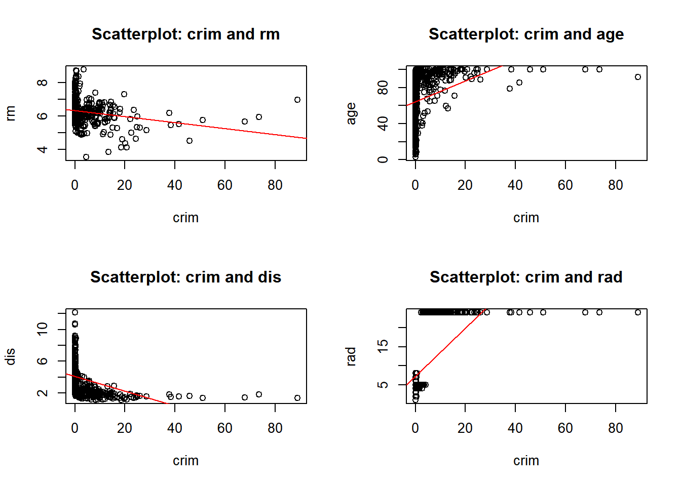
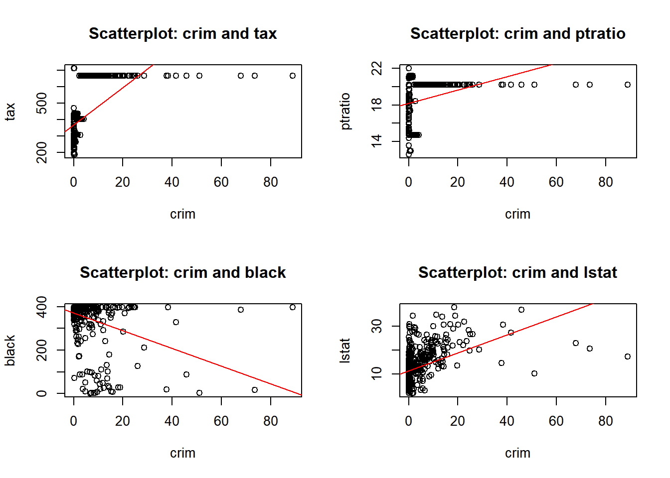
c) Are any of the predictors associated with per capita crime rate? If so, explain the relationship.
par(mfrow =c(2, 2)) # Repeating the same as in 'b'for (i in1:length(predictors)) {for (j in (i+1):length(predictors)) {predictor_x <- predictors[i] predictor_y <- predictors[j]if (!is.na(predictor_x) &&!is.na(predictor_y)) {if (predictor_x =="crim"|| predictor_y =="crim") # Checking for crim as a predictor# Repeating the same as in 'b' {plot(Boston[[predictor_x]], Boston[[predictor_y]],xlab = predictor_x, ylab = predictor_y,main =paste("Scatterplot:", predictor_x, "and", predictor_y))if (predictor_x =="crim") {abline(lm(Boston[[predictor_y]] ~ Boston[[predictor_x]]), col ="red")}}}}}
Yes, there are predictors associated with the per capita crime rate. The following observation where made from the plots above, I also used the linear regression line to help me.
Negative correlation: - crim and zn: There’s a slight negative correlation. - crim and dis: There’s a negative correlation. - crim and black: There’s a negative correlation. - crim and medv: There’s a negative correlation. - crim and indus: There’s a positive correlation.
Positive correlation: - crim and nox: There’s a positive correlation.
- crim and rm: There’s a slight negative correlation. - crim and age: There’s a positive correlation.
- crim and rad: There’s a positive correlation.
- crim and tax: There’s a positive correlation.
- crim and ptratio: There’s a slight positive correlation. - crim and lstat: There’s a positive correlation.
No correlation: - crim and chas: There’s no clear correlation.
In conclusion the plots suggest that areas with higher nitrogen oxide/pollution, industrial areas, older homes, accessibility to radial highways, taxes, and lower status of population are likely to have higher crime rates. On the other hand, areas with more residential land zoning, larger homes, greater distance to five employment centers, and black population tend to have lower crime rates.
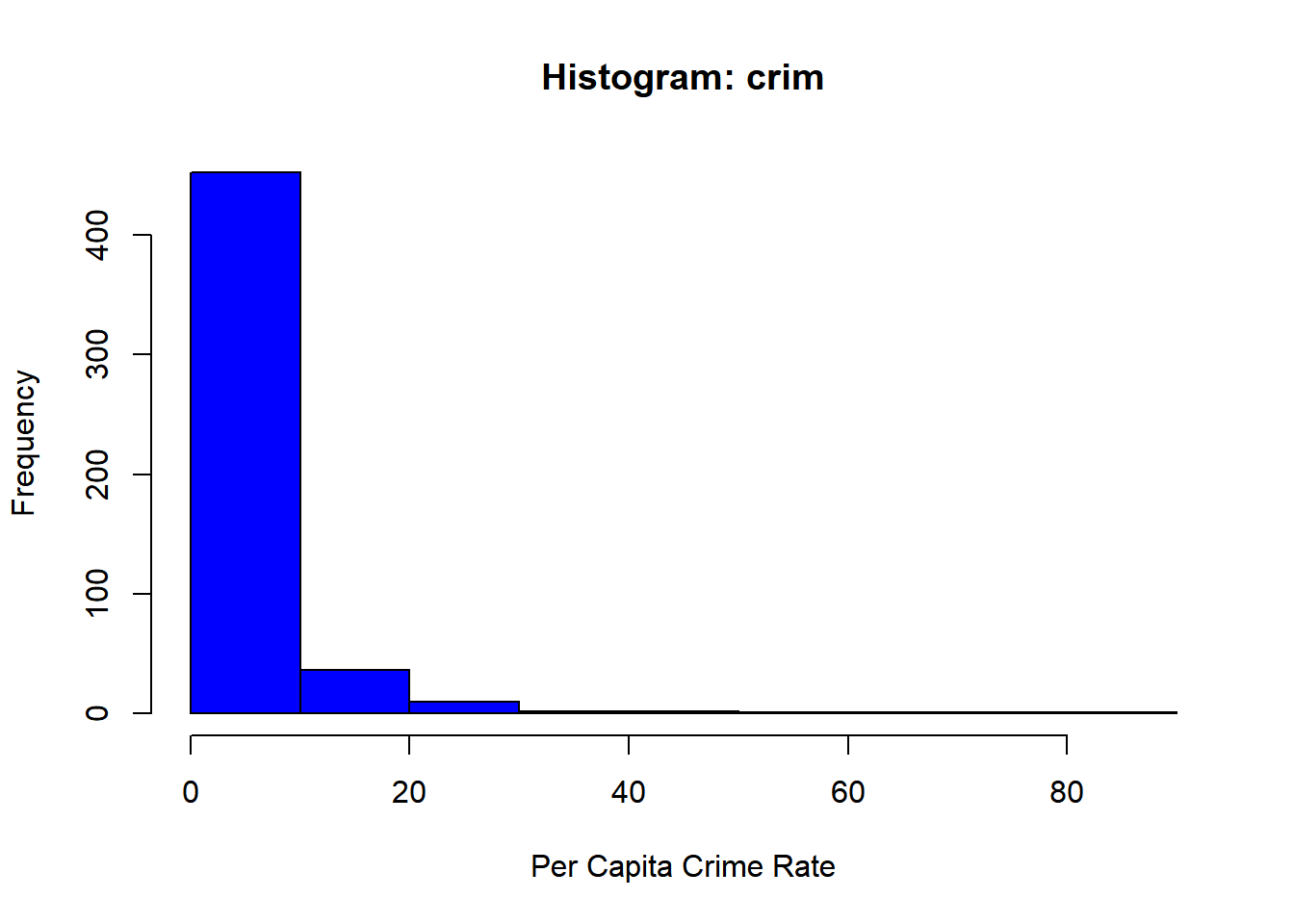
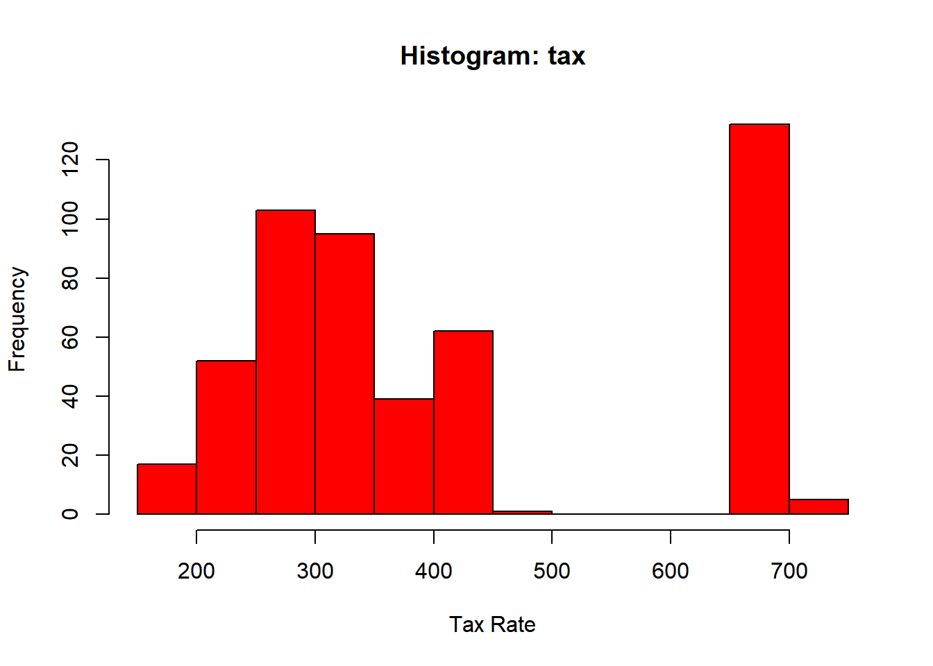
d) Do any of the census tracts of Boston appear to have particularly high crime rates? Tax rates? Comment on the range of each predictor.
hist(Boston$crim, main ="Histogram: crim", xlab ="Per Capita Crime Rate", col ="blue")
hist(Boston$tax, main ="Histogram: tax", xlab ="Tax Rate", col ="red")
# census tracts with high crime rates and tax rateshigh_crime =quantile(Boston$crim, 0.95) high_tax =quantile(Boston$tax, 0.95) high_crime_tracts = Boston[Boston$crim > high_crime, ]high_tax_tracts = Boston[Boston$tax > high_tax, ]rangecrim =range(Boston$crim, na.rm =TRUE)rangetax =range(Boston$tax, na.rm =TRUE)
According to the output there exist census tracts with high crime rates and tax rates, especially in the top 5%. The per capita crime rate ranges from 0.00632 to 88.97620, and the property tax rate range from 187 to 711. This just tells me that there are significant variability for both predictors.
# range of each predictorpredictor_ranges <-apply(Boston, 2, range)predictor_ranges
According to the output there exist census tracts with high crime rates and tax rates, especially in the top 5%. The per capita crime rate ranges from 0.00632 to 88.97620, and the property tax rate range from 187 to 711. This just tells me that there are significant variability for both predictors. In addition to the census tract associated with high crime rates and tax rates, we can also note the rest of the predictors.
Zn-proportion of residential land zoned rate range: 0 to 100
indus-proportion of non-retail business acres per town rate range: 0.46 to 27.74
chas-Charles River rate range: 0 to 1
nox-nitrogen oxides concentration rate range: 0.385 to 0.871 (parts per 10 million)
rm-average number of rooms rate range: 3.561 to 8.780
age-older home rate range: 2.9 to 100
dis-distances to employment centres rate range: 1.1296 to 12.1265
rad-accessibility to radial highways: 1 to 24
ptratio-pupil-teacher ratio by town rate range: 12.6 to 22
black-proportion of black population: 0.32 to 396.90
lstat-lower status of the population rate range: 1.73 to 37.97
medv-median value of owner-occupied rate range: 5 to 50
Just reiterating what was previously stated, these predictors demonstrate that there is significant variability.
e) How many of the census tracts in this data set bound the Charles river?
tracts_chas =sum(Boston$chas ==1)tracts_chas
[1] 35
Since, the predictor chas - Charles River, 1 is if tract bounds river. They’re 35 census tracts.
(f) What is the median pupil-teacher ratio among the towns in this data set?
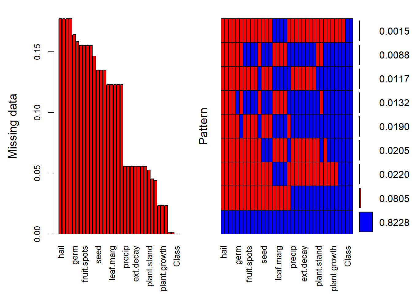
The soybean data can also be found at the UC Irvine Machine Learning Repository. Data were collected to predict disease in 683 soybeans. The 35 predictors are mostly categorical and include information on the environmental conditions (e.g., temperature, precipitation) and plant conditions (e.g., left spots, mold growth). The outcome labels consist of 19 distinct classes.
library(VIM)
Warning: package 'VIM' was built under R version 4.3.3
Loading required package: colorspace
VIM is ready to use.
Suggestions and bug-reports can be submitted at: https://github.com/statistikat/VIM/issues
Attaching package: 'VIM'
The following object is masked from 'package:datasets':

    sleep
library(mice)
Warning: package 'mice' was built under R version 4.3.3
Attaching package: 'mice'
The following object is masked from 'package:kernlab':

    convergence
The following object is masked from 'package:stats':

    filter
The following objects are masked from 'package:base':

    cbind, rbind
library(mlbench)
data(Soybean)
?Soybean
a) Investigate the frequency distributions for the categorical predictors. Are any of the distributions degenerate in the ways discussed earlier in this chapter?
According to the result, the Soybean dataset has no predictors that are degenerate.
b) Roughly 18 % of the data are missing. Are there particular predictors that are more likely to be missing? Is the pattern of missing data related to the classes?
The highest proportion of missing data are as follows:
Hail - 17.7% Server - 17.7% Seed.tmt - 17.7% Germ - 16.4% lodging - 17.7% There are other in the 15% range, and in the 14%, and so on.
Most of the variables seem to be missing data, you have some variables that are not missing (class, and leaves). After looking at the visualization, the missing data does not have a relationship to classes.
c) Develop a strategy for handling missing data, either by eliminating predictors or imputation.
missing_na <-colSums(is.na(Soybean))# Identify predictors with more than 99 missing valuespredictors_removed <-names(missing_na[missing_na >99])# Create a new dataset, now without the predictors that have more than 99 missing valuesSoybean_new <- Soybean[, !(names(Soybean) %in% predictors_removed)]# Summary of the cleaned datasetsummary(Soybean_new)
Explanation: Initially during part a, when I ran this model, I noticed variables that higher amounts of missing data. I decided to remove predictors that had more than 100 missing values and removing them accordingly. This way I can remove any variables that exceeds a specific number of missing values. Finally I create a new dataset that can be used for future analysis.
Brodnjak-Vonina et al. (2005) develop a methodology for food laboratories to determine the type of oil from a sample. In their procedure, they used a gas chromatograph (an instrument that separates chemicals in a sample) to measure seven different fatty acids in an oil. These measurements would then be used to predict the type of oil in food samples. To create their model, they used 96 samples2 of seven types of oils.
These data can be found in the caret package using data(oil). The oil types are contained in a factor variable called oilType. The types are pumpkin (coded as A), sunflower (B), peanut (C), olive (D), soybean (E), rapeseed (F) and corn (G). In R,
a) Use the sample function in base R to create a completely random sample of 60 oils. How closely do the frequencies of the random sample match the original samples? Repeat this procedure several times of understand the variation in the sampling process.
set.seed(123)random_sample <-sample(oilType, 60, replace =FALSE)# Comparing frequencies for the random sample to the original datarandom <-table(random_sample)original <-table(oilType)print("Original Frequencies:")
[1] "Original Frequencies:"
print(original)
oilType
 A  B  C  D  E  F  G
37 26  3  7 11 10  2
cat("\n\n")
print("Random Sample Frequencies:")
[1] "Random Sample Frequencies:"
print(random)
random_sample
 A  B  C  D  E  F  G
24 17  3  3  6  5  2
The random sample has the same frequencies for: C and G.
The random sample has lower frequencies for: A,B, D, E and F.
b) Use the caret package function createDataPartition to create a stratified random sample. How does this compare to completely random samples?
# Following same process as "a"set.seed(123)# creating stratified random samplestratified_sample <-createDataPartition(y = oilType, p =0.1, list =FALSE)stratified_data <- oilType[stratified_sample] stratified_data_df <-as.data.frame(stratified_data)table_stratified <-table(stratified_data_df)cat("Original Frequencies:\n")
The values in the statified sample are much lower than the random sample. This is in part due to the stratified refined method, while the random sample looks at all variables within the dataset at random.
c) With such a small samples size, what are the options for determining performance of the model? Should a test set be used?
Methods such as K-fold, along with the train-test split method, could be an option for determining performance of the refined model.
d) One method for understanding the uncertainty of a test set is to use a confidence interval. To obtain a confidence interval for the overall accuracy, the based R function binom.test can be used. It requires the user to input the number of samples and the number correctly classified to calculate the interval. For example, suppose a test set sample of 20 oil samples was set aside and 76 were used for model training. For this test set size and a model that is about 80 % accurate (16 out of 20 correct), the confidence interval would be computed using
    Exact binomial test

data:  16 and 20
number of successes = 16, number of trials = 20, p-value = 0.01182
alternative hypothesis: true probability of success is not equal to 0.5
95 percent confidence interval:
 0.563386 0.942666
sample estimates:
probability of success
                   0.8
In this case, the width of the 95% confidence interval is 37.9 %, and accuracy 80%.
Try different samples sizes and accuracy rates to understand the trade-off between the uncertainty in the results, the model performance, and the test set size.
    Exact binomial test

data:  41 and 50
number of successes = 41, number of trials = 50, p-value = 5.614e-06
alternative hypothesis: true probability of success is not equal to 0.5
95 percent confidence interval:
 0.6856306 0.9142379
sample estimates:
probability of success
                  0.82
In this case, the width of the 95% confidence interval is 22.9% and accuracy 82%
    Exact binomial test

data:  90 and 100
number of successes = 90, number of trials = 100, p-value < 2.2e-16
alternative hypothesis: true probability of success is not equal to 0.5
95 percent confidence interval:
 0.8237774 0.9509953
sample estimates:
probability of success
                   0.9
In this case, the width of the 95% confidence interval is 12.7%, and accuracy 90%
In conclusion, I noticed that as the sample size increases it reduces the confidence level. However, as the accuracy rate increases it tends to reduce the interval width.
Briefly discuss what is the bias-variance tradeoff in statistics and predictive modeling.
The bias-variance tradeoff is when we chose lower bias which increases variance or lower variance increases bias. The objective is to find a good balance meaning that both bias and variance are at minimal.
Predicting Fat Content in Meat Using IR Spectroscopy and Machine Learning: A Comparative Study of Predictive Models
Infrared (IR) spectroscopy technology is used to determine the chemical makeup of a substance. The theory of IR spectroscopy holds that unique molecular structures absorb IR frequencies differently. In practice a spectrometer fires a series of IR frequencies into a sample material, and the device measures the absorbance of the sample at each individual frequency. This series of measurements creates a spectrum profile which can then be used to determine the chemical makeup of the sample material.
A Tecator Infratec Food and Feed Analyzer instrument was used to analyze 215 samples of meat across 100 frequencies. A sample of these frequency profiles is displayed in Fig. 6.20. In addition to an IR profile, analytical chemistry determined the percent content of water, fat, and protein for each sample. If we can establish a predictive relationship between IR spectrum and fat content, then food scientists could predict a sample’s fat content with IR instead of using analytical chemistry. This would provide costs savings, since analytical chemistry is a more expensive, time-consuming process.
a) Start R and use these commands to load the data:
The matrix absorp contains the 100 absorbance values for the 215 samples, while matrix endpoints contain the percent of moisture, fat, and protein in columns 1–3, respectively. To be more specific
b) Split the data into a training and a test set the response of the percentage of protein, pre-process the data as appropriate.
set.seed(123)index <-createDataPartition(protein, p =0.7, list =FALSE)train_data <-data.frame(absorp[index, ], protein = protein[index])test_data <-data.frame(absorp[-index, ], protein = protein[-index])
n_train <-nrow(train_data)train_pca <-cbind(combined_pca[1:n_train, ], protein = train_data$protein)test_pca <-cbind(combined_pca[(n_train +1):nrow(combined_data), ], protein = test_data$protein)
c) Build at least three models described Chapter 6: ordinary least squares, PCR, PLS, Ridge, and ENET. For those models with tuning parameters, what are the optimal values of the tuning parameter(s)?
Ordinary Least Squares (OLS):
set.seed(123)ols_model <-train(protein ~ ., data = train_pca, method ="lm")ols_model
Linear Regression

152 samples
 20 predictor

No pre-processing
Resampling: Bootstrapped (25 reps)
Summary of sample sizes: 152, 152, 152, 152, 152, 152, ...
Resampling results:

  RMSE       Rsquared   MAE
  0.7268192  0.9450398  0.5549019

Tuning parameter 'intercept' was held constant at a value of TRUE
Principal Component Analysis

152 samples
100 predictors

No pre-processing
Resampling: Cross-Validated (10 fold)
Summary of sample sizes: 136, 137, 137, 137, 136, 138, ...
Resampling results across tuning parameters:

  ncomp  RMSE      Rsquared   MAE
  1      2.966122  0.1570382  2.520911
  2      2.854048  0.1843866  2.337577
  3      2.316586  0.4545058  1.848556

RMSE was used to select the optimal model using the smallest value.
The final value used for the model was ncomp = 3.
Partial Least Squares

152 samples
100 predictors

No pre-processing
Resampling: Cross-Validated (10 fold)
Summary of sample sizes: 136, 137, 137, 137, 136, 138, ...
Resampling results across tuning parameters:

  ncomp  RMSE      Rsquared   MAE
  1      2.959109  0.1580897  2.511023
  2      2.256430  0.5094219  1.788162
  3      1.743833  0.6963113  1.291007

RMSE was used to select the optimal model using the smallest value.
The final value used for the model was ncomp = 3.
Partial Least Squares (PLS):
ncomp: 3
RMSE: 1.743833
R-squared: 0.6963113
MAE: 1.291007
d) Build nonlinear models in Chapter 7: SVM, neural network, MARS, and KNN models. Since neural networks are especially sensitive to highly correlated predictors, does pre-processing using PCA help the model? For those models with tuning parameters, what are the optimal values of the tuning parameter(s)?
Support Vector Machines with Radial Basis Function Kernel

152 samples
100 predictors

No pre-processing
Resampling: Cross-Validated (10 fold)
Summary of sample sizes: 136, 137, 137, 137, 136, 138, ...
Resampling results across tuning parameters:

  C       RMSE      Rsquared   MAE
    0.25  2.683055  0.3123868  2.126981
    0.50  2.431071  0.4167549  1.921845
    1.00  2.135216  0.5501123  1.656360
    2.00  1.934330  0.6259364  1.506506
    4.00  1.812361  0.6698215  1.397221
    8.00  1.744285  0.6980792  1.333155
   16.00  1.717343  0.7085363  1.317764
   32.00  1.676734  0.7178974  1.272854
   64.00  1.805285  0.6829508  1.316395
  128.00  1.910920  0.6787767  1.327847

Tuning parameter 'sigma' was held constant at a value of 0.05200074
RMSE was used to select the optimal model using the smallest value.
The final values used for the model were sigma = 0.05200074 and C = 32.
Multivariate Adaptive Regression Spline
152 samples
100 predictors
No pre-processing
Resampling: Cross-Validated (10 fold)
Summary of sample sizes: 136, 137, 137, 137, 136, 138, ...
Resampling results across tuning parameters:
nprune RMSE Rsquared MAE
2 2.854067 0.1814645 2.3879962
15 1.212796 0.8517258 0.9221938
28 1.357497 0.8313863 0.9689615
Tuning parameter 'degree' was held constant at a value of 1
RMSE was used to select the optimal model using the smallest value.
The final values used for the model were nprune = 15 and degree = 1.
k-Nearest Neighbors
152 samples
100 predictors
No pre-processing
Resampling: Cross-Validated (10 fold)
Summary of sample sizes: 136, 137, 137, 137, 136, 138, ...
Resampling results across tuning parameters:
k RMSE Rsquared MAE
5 2.300655 0.4780876 1.909033
7 2.453521 0.3946490 2.032608
9 2.511651 0.3773289 2.075073
11 2.550576 0.3616637 2.087163
13 2.619400 0.3441352 2.145169
15 2.654108 0.3080377 2.188281
17 2.716741 0.2774054 2.239304
19 2.716383 0.2760947 2.254749
21 2.773202 0.2384392 2.297991
23 2.789007 0.2262430 2.320930
RMSE was used to select the optimal model using the smallest value.
The final value used for the model was k = 5.
kNN:
k: 5
RMSE: 2.300655
squared: 0.4780876
MAE: 1.909033
e) Which model from parts c) and d) has the best predictive ability? Is any model significantly better or worse than the others?
Model
RMSE
Rsquared
MAE
Rank
OLS - Linear Regression
0.7268192
0.9450398
0.5549019
1
Principal Component Regression (PCR)
2.316586
0.4545058
1.848556
6
Partial Least Squares (PLS)
1.743833
0.6963113
1.291007
4
SVM
1.676734
0.7178974
1.272854
3
Neural Network
16.94374
NA
16.66501
7
MARS
1.212796
0.8517258
0.9221938
2
kNN
2.300655
0.478087
1.909033
5
In conclusion, I have ranked the models according to the criteria of lowest RMSE, and lowest MAE, and high rsquared. The OLS - Linear Regression outperforms all other models, followed by the MARS. The Nueral Network model performs the worst out of all the other models as it has the highest RMSE and the rsquared is not available.
Developing a model to predict permeability (see Sect. 1.4 of the textbook) could save significant resources for a pharmaceutical company, while at the same time more rapidly identifying molecules that have a sufficient permeability to become a drug:
a) Start R and use these commands to load the data:
The matrix fingerprints contains the 1,107 binary molecular predictors for the 165 compounds, while permeability contains permeability response:
b) The fingerprint predictors indicate the presence or absence of substructures of a molecule and are often sparse meaning that relatively few of the molecules contain each substructure. Filter out the predictors that have low frequencies using the nearZeroVar function from the caret package. How many predictors are left for modeling?
c) Split the data into a training and a test set, pre-process the data, and tune a PLS model. How many latent variables are optimal and what is the corresponding resampled estimate of R2?
set.seed(123)index <-createDataPartition(permeability, p =0.7, list =FALSE)train_data <- filtered_fingerprints[index, ]train_permeability <- permeability[index]test_data <- filtered_fingerprints[-index, ]test_permeability <- permeability[-index]# Preprocess the data (center and scale)preProcValues <-preProcess(train_data, method =c("center", "scale"))train_data_transformed <-predict(preProcValues, train_data)test_data_transformed <-predict(preProcValues, test_data)
Partial Least Squares
117 samples
388 predictors
No pre-processing
Resampling: Cross-Validated (10 fold)
Summary of sample sizes: 105, 105, 106, 105, 105, 105, ...
Resampling results across tuning parameters:
ncomp RMSE Rsquared MAE
1 13.36436 0.3433889 10.474224
2 12.30920 0.4595424 8.621998
3 12.79841 0.4713902 9.518968
4 13.01506 0.4586135 9.759753
5 13.50115 0.4188773 9.868189
6 13.28765 0.4391301 9.680872
7 12.89540 0.4604643 9.314659
8 12.82966 0.4653079 9.399587
9 12.94528 0.4583512 9.434668
10 13.30683 0.4341421 9.892463
RMSE was used to select the optimal model using the smallest value.
The final value used for the model was ncomp = 2.
Support Vector Machines with Radial Basis Function Kernel
117 samples
388 predictors
No pre-processing
Resampling: Cross-Validated (10 fold)
Summary of sample sizes: 105, 105, 106, 105, 105, 105, ...
Resampling results across tuning parameters:
C RMSE Rsquared MAE
0.25 13.31509 0.4937223 8.559747
0.50 12.03042 0.5011860 7.954428
1.00 11.71028 0.5103354 7.664866
2.00 11.87293 0.4929464 7.786952
4.00 12.17146 0.4658056 8.201456
8.00 12.33716 0.4474256 8.447651
16.00 12.33661 0.4453930 8.476095
32.00 12.29978 0.4482620 8.468869
64.00 12.27952 0.4499855 8.465674
128.00 12.27952 0.4499855 8.465674
Tuning parameter 'sigma' was held constant at a value of 0.003241275
RMSE was used to select the optimal model using the smallest value.
The final values used for the model were sigma = 0.003241275 and C = 1.
Warning: model fit failed for Fold04: lambda=0.0000000 Error in if (zmin < gamhat) { : missing value where TRUE/FALSE needed
Warning in nominalTrainWorkflow(x = x, y = y, wts = weights, info = trainInfo,
: There were missing values in resampled performance measures.
ridge2_model
Ridge Regression
117 samples
388 predictors
No pre-processing
Resampling: Cross-Validated (10 fold)
Summary of sample sizes: 105, 105, 106, 105, 105, 105, ...
Resampling results across tuning parameters:
lambda RMSE Rsquared MAE
0.0000000000 22.42497 0.27702987 15.70016
0.0001000000 6615.25285 0.08396519 3563.99122
0.0002371374 99671.84144 0.08457611 62604.59123
0.0005623413 170244.42077 0.14306870 104949.49993
0.0013335214 13949.49087 0.14095413 8819.60573
0.0031622777 1338.29409 0.09027590 926.17683
0.0074989421 4869.57307 0.19911169 3391.43119
0.0177827941 17.66500 0.25592818 12.61336
0.0421696503 15.69511 0.31773516 11.39005
0.1000000000 14.70937 0.37493137 10.76181
RMSE was used to select the optimal model using the smallest value.
The final value used for the model was lambda = 0.1.
Warning: model fit failed for Fold04: fraction=0.9 Error in if (zmin < gamhat) { : missing value where TRUE/FALSE needed
Warning in nominalTrainWorkflow(x = x, y = y, wts = weights, info = trainInfo,
: There were missing values in resampled performance measures.
lasso2_model
The lasso
117 samples
388 predictors
No pre-processing
Resampling: Cross-Validated (10 fold)
Summary of sample sizes: 105, 105, 106, 105, 105, 105, ...
Resampling results across tuning parameters:
fraction RMSE Rsquared MAE
0.1000000 12.76949 0.4681541 9.532476
0.1888889 13.75236 0.4031430 9.879639
0.2777778 14.64878 0.3661843 10.403824
0.3666667 15.57692 0.3421552 11.066913
0.4555556 16.62051 0.3177241 11.791049
0.5444444 17.77760 0.3013368 12.521844
0.6333333 18.87893 0.2964326 13.284076
0.7222222 20.07676 0.2902689 14.162004
0.8111111 21.22992 0.2871456 14.928141
0.9000000 21.91715 0.2806466 15.326569
RMSE was used to select the optimal model using the smallest value.
The final value used for the model was fraction = 0.1.
f) Would you recommend any of your models to replace the permeability laboratory experiment?
According to the table above, SVM has the lowest RMSE, and MAE, this model has less of a possibility to give us an error. However, the Ridge Regression model has the highest rquared, which simply means that this model can explain the highest variance out of the other models. Now, my recommendation, would be to use the SVM model for this laboratory experiment, the reason is because it has the lowest RMSE and MAE, and a decent amount of variance can be explained by this model.
Return to the permeability problem outlined in Problem 2. Train several nonlinear regression models and evaluate the resampling and test set performance.
a) Which nonlinear regression model that we learned in Chapter 7 gives the optimal resampling and test set performance?
NONLINEAR
RMSE
Rsquared
MAE
SVM
10.5483639
0.4394321
7.1154118
Neural Network
12.731659
0.197259
9.597258
MARS
11.8764033
0.3239788
7.5933958
kNN
10.5121448
0.4547602
6.9931969
The kNN Model gives the optimal resampling and test set performance, because it has the lowest RMSE and the highest R-squared compared to the others.
b) Do any of the nonlinear models outperform the optimal linear model you previously developed in Problem 2? If so, what might this tell you about the underlying relationship between the predictors and the response?
NONLINEAR
RMSE
Rsquared
MAE
SVM
10.5483639
0.4394321
7.1154118
Neural Network
12.731659
0.197259
9.597258
MARS
11.8764033
0.3239788
7.5933958
kNN
10.5121448
0.4547602
6.9931969
Other Models Ran in Q2
RMSE
Rsquared
MAE
Test_set_rsquared
PLS Model
12.30920
0.4595424
8.621998
0.3819407
Ridge Rigression
14.70937
0.3749313
10.76181
0.5311375
Lasso Regression
12.76949
0.4681541
9.532476
0.4573928
SVM
11.71028
0.5103354
7.664866
0.4394321
Yes, the best model so far is the kNN model, which seems to outperform all the other models, this model has the lowest RMSE and MAE, and its rsquared value is not the lowest. This highlights the relationship between predictors and the response variables are nonlinear.
c) Would you recommend any of the models you have developed to replace the permeability laboratory experiment?
Based on the results, I recommend using the kNN model. This model demonstrates the lowest RMSE and MAE, indicating it has the smallest error and provides the most accurate predictions. Additionally, it has one of the higher R-squared values, suggesting it effectively explains the variability in the data.
Analyzing and Predicting Oil Types and Customer Churn Using Machine Learning Techniques
Warning: package 'rsample' was built under R version 4.3.3
Attaching package: 'rsample'
The following object is masked from 'package:e1071':
permutations
library(recipes)
Warning: package 'recipes' was built under R version 4.3.3
Attaching package: 'recipes'
The following object is masked from 'package:stringr':
fixed
The following object is masked from 'package:VIM':
prepare
The following object is masked from 'package:stats4':
update
The following object is masked from 'package:stats':
step
library(rpart)library(ranger)
Warning: package 'ranger' was built under R version 4.3.3
Attaching package: 'ranger'
The following object is masked from 'package:randomForest':
importance
library(nnet)library(caret)library(yardstick)
Warning: package 'yardstick' was built under R version 4.3.3
Attaching package: 'yardstick'
The following object is masked from 'package:readr':
spec
The following objects are masked from 'package:caret':
precision, recall, sensitivity, specificity
Warning: package 'xgboost' was built under R version 4.3.3
Attaching package: 'xgboost'
The following object is masked from 'package:dplyr':
slice
In Homework 1, Problem 3, we described a data set which contained 96 oil samples each from one of seven types of oils (pumpkin, sunflower, peanut, olive, soybean, rapeseed, and corn). Gas chromatography was performed on each sample and the percentage of each type of 7 fatty acids was determined. We would like to use these data to build a model that predicts the type of oil based on a sample’s fatty acid percentages. These data can be found in the caret package using data(oil). The oil types are contained in a factor variable called oilType. The types are pumpkin (coded as A), sunflower (B), peanut (C), olive (D), soybean (E), rapeseed (F) and corn (G). In R
Given the classification imbalance in oil Type, describe how you would create a training and testing set.
# Convert the fatty acid compositions into a data frameoil_data <-as.data.frame(fattyAcids)oil_data$oilType <- oilType# Set seed for reproducibilityset.seed(123)# Split the data using stratified samplingtrain_index <-createDataPartition(oil_data$oilType, p =0.7, list =FALSE)train_data <- oil_data[train_index, ]test_data <- oil_data[-train_index, ]# Pre-process the data: Centering and ScalingpreProcValues <-preProcess(train_data[,-ncol(train_data)], method =c("center", "scale"))train_data[,-ncol(train_data)] <-predict(preProcValues, train_data[,-ncol(train_data)])test_data[,-ncol(test_data)] <-predict(preProcValues, test_data[,-ncol(test_data)])# Control for cross-validationctrl <-trainControl(method ="cv", number =10, classProbs =TRUE, summaryFunction = multiClassSummary)# Check for missing values in the datasetcolSums(is.na(train_data))
# Remove rows with missing valuestrain_data_clean <-na.omit(train_data)# Impute missing values using the medianpreProcess_missing <-preProcess(train_data, method ='medianImpute')train_data_clean <-predict(preProcess_missing, train_data)
Which classification statistic would you choose to optimize for this problem and why?
I would choose the F1 score in cases where the classes are imbalanced. The objective is to achieve a balance between precision and recall.
Split the data into a training and a testing set, pre-process the data, and build models and tune them via resampling described in Chapter 12. Clearly list the models under consideration and the corresponding tuning parameters of the models.
Warning in nominalTrainWorkflow(x = x, y = y, wts = weights, info = trainInfo,
: There were missing values in resampled performance measures.
knn_model
k-Nearest Neighbors
70 samples
7 predictor
7 classes: 'A', 'B', 'C', 'D', 'E', 'F', 'G'
No pre-processing
Resampling: Cross-Validated (10 fold)
Summary of sample sizes: 62, 61, 62, 65, 63, 62, ...
Resampling results across tuning parameters:
k logLoss AUC prAUC Accuracy Kappa Mean_F1
5 0.5583384 0.9919921 0.01388889 0.9375000 0.9195499 NaN
7 0.2130499 0.9974206 0.01708333 0.9138889 0.8913839 NaN
9 0.2846983 0.9926091 0.01504630 0.8902778 0.8606707 NaN
11 0.3528189 0.9904927 0.01430556 0.8500000 0.7986789 NaN
13 0.4069273 0.9866567 0.04625000 0.8333333 0.7649739 NaN
15 0.4571756 0.9891865 0.06750000 0.8208333 0.7493668 NaN
17 0.5034627 0.9847983 0.07888889 0.7629365 0.6623458 NaN
19 0.5718785 0.9844444 0.06222222 0.7629365 0.6633254 NaN
21 0.6450366 0.9800893 0.10847222 0.7179365 0.5943018 NaN
23 0.7030457 0.9753274 0.15388889 0.7054365 0.5779753 NaN
Mean_Sensitivity Mean_Specificity Mean_Pos_Pred_Value Mean_Neg_Pred_Value
NaN 0.9879592 NaN NaN
NaN 0.9852891 NaN NaN
NaN 0.9805272 NaN NaN
NaN 0.9712585 NaN NaN
NaN 0.9652041 NaN NaN
NaN 0.9632993 NaN NaN
NaN 0.9493878 NaN NaN
NaN 0.9497279 NaN NaN
NaN 0.9405612 NaN NaN
NaN 0.9381803 NaN NaN
Mean_Precision Mean_Recall Mean_Detection_Rate Mean_Balanced_Accuracy
NaN NaN 0.1339286 NaN
NaN NaN 0.1305556 NaN
NaN NaN 0.1271825 NaN
NaN NaN 0.1214286 NaN
NaN NaN 0.1190476 NaN
NaN NaN 0.1172619 NaN
NaN NaN 0.1089909 NaN
NaN NaN 0.1089909 NaN
NaN NaN 0.1025624 NaN
NaN NaN 0.1007766 NaN
Accuracy was used to select the optimal model using the largest value.
The final value used for the model was k = 5.
# weights: 63 (48 variable)
initial value 120.646429
iter 10 value 0.230492
iter 20 value 0.009305
iter 30 value 0.005935
iter 40 value 0.003696
iter 50 value 0.000954
iter 60 value 0.000826
iter 70 value 0.000260
iter 80 value 0.000245
final value 0.000060
converged
# weights: 63 (48 variable)
initial value 120.646429
iter 10 value 13.646415
iter 20 value 12.851693
final value 12.849291
converged
# weights: 63 (48 variable)
initial value 120.646429
iter 10 value 0.426250
iter 20 value 0.207953
iter 30 value 0.168443
iter 40 value 0.149413
iter 50 value 0.139491
iter 60 value 0.133972
iter 70 value 0.127703
iter 80 value 0.124725
iter 90 value 0.122750
iter 100 value 0.121841
final value 0.121841
stopped after 100 iterations
# weights: 63 (48 variable)
initial value 118.700519
iter 10 value 0.649572
iter 20 value 0.072909
iter 30 value 0.019004
iter 40 value 0.003326
iter 50 value 0.000645
iter 60 value 0.000422
iter 70 value 0.000364
final value 0.000098
converged
# weights: 63 (48 variable)
initial value 118.700519
iter 10 value 13.670469
iter 20 value 12.717571
final value 12.717563
converged
# weights: 63 (48 variable)
initial value 118.700519
iter 10 value 0.686614
iter 20 value 0.158090
iter 30 value 0.125404
iter 40 value 0.118784
iter 50 value 0.114113
iter 60 value 0.112865
iter 70 value 0.110695
iter 80 value 0.109572
iter 90 value 0.109285
iter 100 value 0.109183
final value 0.109183
stopped after 100 iterations
# weights: 63 (48 variable)
initial value 120.646429
iter 10 value 1.152097
iter 20 value 0.109926
iter 30 value 0.001534
iter 40 value 0.000261
final value 0.000067
converged
# weights: 63 (48 variable)
initial value 120.646429
iter 10 value 14.882114
iter 20 value 13.391351
final value 13.391006
converged
# weights: 63 (48 variable)
initial value 120.646429
iter 10 value 1.193110
iter 20 value 0.224979
iter 30 value 0.168419
iter 40 value 0.160797
iter 50 value 0.156729
iter 60 value 0.153777
iter 70 value 0.150874
iter 80 value 0.149621
iter 90 value 0.148691
iter 100 value 0.148334
final value 0.148334
stopped after 100 iterations
# weights: 63 (48 variable)
initial value 126.484160
iter 10 value 1.375234
iter 20 value 0.124856
iter 30 value 0.012044
iter 40 value 0.002572
final value 0.000097
converged
# weights: 63 (48 variable)
initial value 126.484160
iter 10 value 15.628076
iter 20 value 13.989692
final value 13.989554
converged
# weights: 63 (48 variable)
initial value 126.484160
iter 10 value 1.417908
iter 20 value 0.245160
iter 30 value 0.180883
iter 40 value 0.170537
iter 50 value 0.167035
iter 60 value 0.162098
iter 70 value 0.157875
iter 80 value 0.156208
iter 90 value 0.154991
iter 100 value 0.154037
final value 0.154037
stopped after 100 iterations
# weights: 63 (48 variable)
initial value 122.592339
iter 10 value 1.160417
iter 20 value 0.162686
iter 30 value 0.015871
iter 40 value 0.001935
iter 50 value 0.000669
final value 0.000081
converged
# weights: 63 (48 variable)
initial value 122.592339
iter 10 value 15.295508
iter 20 value 13.937812
final value 13.936771
converged
# weights: 63 (48 variable)
initial value 122.592339
iter 10 value 1.211200
iter 20 value 0.266794
iter 30 value 0.174726
iter 40 value 0.165736
iter 50 value 0.162175
iter 60 value 0.157912
iter 70 value 0.155364
iter 80 value 0.153778
iter 90 value 0.152625
iter 100 value 0.151735
final value 0.151735
stopped after 100 iterations
# weights: 63 (48 variable)
initial value 120.646429
iter 10 value 0.982411
iter 20 value 0.066584
iter 30 value 0.011904
iter 40 value 0.002347
iter 50 value 0.001356
final value 0.000097
converged
# weights: 63 (48 variable)
initial value 120.646429
iter 10 value 17.094756
iter 20 value 13.621311
final value 13.620050
converged
# weights: 63 (48 variable)
initial value 120.646429
iter 10 value 1.025922
iter 20 value 0.188570
iter 30 value 0.160388
iter 40 value 0.154288
iter 50 value 0.149946
iter 60 value 0.145432
iter 70 value 0.143887
iter 80 value 0.141985
iter 90 value 0.140837
iter 100 value 0.140255
final value 0.140255
stopped after 100 iterations
# weights: 63 (48 variable)
initial value 120.646429
iter 10 value 0.201740
iter 20 value 0.036329
iter 30 value 0.015300
iter 40 value 0.006737
iter 50 value 0.001509
iter 60 value 0.001034
iter 70 value 0.000403
iter 80 value 0.000390
final value 0.000095
converged
# weights: 63 (48 variable)
initial value 120.646429
iter 10 value 15.237850
iter 20 value 13.504443
final value 13.503651
converged
# weights: 63 (48 variable)
initial value 120.646429
iter 10 value 0.345888
iter 20 value 0.205508
iter 30 value 0.195911
iter 40 value 0.175069
iter 50 value 0.161029
iter 60 value 0.154607
iter 70 value 0.150725
iter 80 value 0.149049
iter 90 value 0.147205
iter 100 value 0.146646
final value 0.146646
stopped after 100 iterations
# weights: 63 (48 variable)
initial value 124.538250
iter 10 value 1.423335
iter 20 value 0.097869
iter 30 value 0.013049
iter 40 value 0.000310
final value 0.000099
converged
# weights: 63 (48 variable)
initial value 124.538250
iter 10 value 15.998770
iter 20 value 13.988523
final value 13.987954
converged
# weights: 63 (48 variable)
initial value 124.538250
iter 10 value 1.461579
iter 20 value 0.221927
iter 30 value 0.182446
iter 40 value 0.172022
iter 50 value 0.166376
iter 60 value 0.158815
iter 70 value 0.155713
iter 80 value 0.154033
iter 90 value 0.153355
iter 100 value 0.152889
final value 0.152889
stopped after 100 iterations
# weights: 63 (48 variable)
initial value 126.484160
iter 10 value 1.036502
iter 20 value 0.114252
iter 30 value 0.014528
iter 40 value 0.002648
iter 50 value 0.000355
final value 0.000100
converged
# weights: 63 (48 variable)
initial value 126.484160
iter 10 value 14.854834
iter 20 value 13.259516
final value 13.259460
converged
# weights: 63 (48 variable)
initial value 126.484160
iter 10 value 1.076774
iter 20 value 0.208832
iter 30 value 0.157131
iter 40 value 0.147462
iter 50 value 0.144709
iter 60 value 0.143059
iter 70 value 0.140412
iter 80 value 0.139310
iter 90 value 0.138768
iter 100 value 0.138344
final value 0.138344
stopped after 100 iterations
# weights: 63 (48 variable)
initial value 124.538250
iter 10 value 1.127422
iter 20 value 0.120905
iter 30 value 0.019095
iter 40 value 0.000191
final value 0.000076
converged
# weights: 63 (48 variable)
initial value 124.538250
iter 10 value 16.170644
iter 20 value 14.131864
final value 14.130439
converged
# weights: 63 (48 variable)
initial value 124.538250
iter 10 value 1.178679
iter 20 value 0.235910
iter 30 value 0.180086
iter 40 value 0.170725
iter 50 value 0.165276
iter 60 value 0.160358
iter 70 value 0.157981
iter 80 value 0.156756
iter 90 value 0.155457
iter 100 value 0.154352
final value 0.154352
stopped after 100 iterations
Warning in nominalTrainWorkflow(x = x, y = y, wts = weights, info = trainInfo,
: There were missing values in resampled performance measures.
# weights: 63 (48 variable)
initial value 136.213710
iter 10 value 18.641421
iter 20 value 14.337670
final value 14.337620
converged
log_reg_model
Penalized Multinomial Regression
70 samples
7 predictor
7 classes: 'A', 'B', 'C', 'D', 'E', 'F', 'G'
No pre-processing
Resampling: Cross-Validated (10 fold)
Summary of sample sizes: 62, 61, 62, 65, 63, 62, ...
Resampling results across tuning parameters:
decay logLoss AUC prAUC Accuracy Kappa Mean_F1
0e+00 0.5777232 0.9892857 0.2177480 0.9313889 0.9115174 NaN
1e-04 0.4544908 0.9930556 0.2457738 0.9513889 0.9387330 NaN
1e-01 0.1882385 0.9972222 0.2473611 0.9513889 0.9387330 NaN
Mean_Sensitivity Mean_Specificity Mean_Pos_Pred_Value Mean_Neg_Pred_Value
NaN 0.9882993 NaN NaN
NaN 0.9920918 NaN NaN
NaN 0.9920918 NaN NaN
Mean_Precision Mean_Recall Mean_Detection_Rate Mean_Balanced_Accuracy
NaN NaN 0.1330556 NaN
NaN NaN 0.1359127 NaN
NaN NaN 0.1359127 NaN
Accuracy was used to select the optimal model using the largest value.
The final value used for the model was decay = 0.1.
Warning in nominalTrainWorkflow(x = x, y = y, wts = weights, info = trainInfo,
: There were missing values in resampled performance measures.
rf_model
Random Forest
70 samples
7 predictor
7 classes: 'A', 'B', 'C', 'D', 'E', 'F', 'G'
No pre-processing
Resampling: Cross-Validated (10 fold)
Summary of sample sizes: 62, 61, 62, 65, 63, 62, ...
Resampling results across tuning parameters:
mtry logLoss AUC prAUC Accuracy Kappa Mean_F1
1.0 0.2490844 1 0.2522222 0.9625 0.9523009 NaN
2.2 0.1537911 1 0.2188889 0.9750 0.9679487 NaN
3.4 0.1361475 1 0.2147222 0.9750 0.9679487 NaN
4.6 0.1333570 1 0.1791667 0.9550 0.9405111 NaN
5.8 0.1378782 1 0.1583333 0.9550 0.9405111 NaN
7.0 0.1509535 1 0.1455556 0.9550 0.9405111 NaN
Mean_Sensitivity Mean_Specificity Mean_Pos_Pred_Value Mean_Neg_Pred_Value
NaN 0.9934524 NaN NaN
NaN 0.9959184 NaN NaN
NaN 0.9959184 NaN NaN
NaN 0.9933163 NaN NaN
NaN 0.9933163 NaN NaN
NaN 0.9933163 NaN NaN
Mean_Precision Mean_Recall Mean_Detection_Rate Mean_Balanced_Accuracy
NaN NaN 0.1375000 NaN
NaN NaN 0.1392857 NaN
NaN NaN 0.1392857 NaN
NaN NaN 0.1364286 NaN
NaN NaN 0.1364286 NaN
NaN NaN 0.1364286 NaN
Accuracy was used to select the optimal model using the largest value.
The final value used for the model was mtry = 2.2.
Random Forest:
mtry = 2.2
LogLoss: 0.1537911
AUC: 1
prAUC: 0.2188889
Accuracy: 0.9750
Kappa: 0.9679487
Mean_Specificity: 0.9959184
Mean_Detection_Rate: 0.1392857
Summary:
Model
Tuning Parameter
Accuracy
Kappa
AUC
prAUC
k-NN
k = 5
0.9375
0.9195499
0.9920
0.0139
Logistic Regression
decay = 0.1
0.9514
0.9387330
0.9972
0.2474
Random Forest
mtry = 2.2
0.9750
0.9679487
1.0000
0.2189
Conclusion: Out of all the models the Random Forest performs the best with the highest accuracy, Kappa, and AUC score. Then followed by the Logistic Regression model, and the model that performed the worst is the k-NN model. Altogether these models performed well, but the Random Forest out performs the rest of the models.
Of the models presented in this chapter, which performs best on these data? Which oil type does the model most accurately predict? Least accurately predict?
Confusion Matrix and Statistics
Reference
Prediction A B C D E F G
A 10 0 0 0 0 0 0
B 1 7 0 0 0 0 0
C 0 0 0 0 0 0 0
D 0 0 0 2 0 0 0
E 0 0 0 0 3 0 0
F 0 0 0 0 0 3 0
G 0 0 0 0 0 0 0
Overall Statistics
Accuracy : 0.9615
95% CI : (0.8036, 0.999)
No Information Rate : 0.4231
P-Value [Acc > NIR] : 7.058e-09
Kappa : 0.9467
Mcnemar's Test P-Value : NA
Statistics by Class:
Class: A Class: B Class: C Class: D Class: E Class: F
Sensitivity 0.9091 1.0000 NA 1.00000 1.0000 1.0000
Specificity 1.0000 0.9474 1 1.00000 1.0000 1.0000
Pos Pred Value 1.0000 0.8750 NA 1.00000 1.0000 1.0000
Neg Pred Value 0.9375 1.0000 NA 1.00000 1.0000 1.0000
Prevalence 0.4231 0.2692 0 0.07692 0.1154 0.1154
Detection Rate 0.3846 0.2692 0 0.07692 0.1154 0.1154
Detection Prevalence 0.3846 0.3077 0 0.07692 0.1154 0.1154
Balanced Accuracy 0.9545 0.9737 NA 1.00000 1.0000 1.0000
Class: G
Sensitivity NA
Specificity 1
Pos Pred Value NA
Neg Pred Value NA
Prevalence 0
Detection Rate 0
Detection Prevalence 0
Balanced Accuracy NA
kNN:
Accuracy: 0.9615
Kappa: 0.9467
Class A, B, D, E, and F are good.
Class C, and G have no predictions
print(log_reg_cm)
Confusion Matrix and Statistics
Reference
Prediction A B C D E F G
A 10 0 0 0 0 0 0
B 1 7 0 0 0 0 0
C 0 0 0 0 0 0 0
D 0 0 0 2 0 0 0
E 0 0 0 0 3 0 0
F 0 0 0 0 0 3 0
G 0 0 0 0 0 0 0
Overall Statistics
Accuracy : 0.9615
95% CI : (0.8036, 0.999)
No Information Rate : 0.4231
P-Value [Acc > NIR] : 7.058e-09
Kappa : 0.9467
Mcnemar's Test P-Value : NA
Statistics by Class:
Class: A Class: B Class: C Class: D Class: E Class: F
Sensitivity 0.9091 1.0000 NA 1.00000 1.0000 1.0000
Specificity 1.0000 0.9474 1 1.00000 1.0000 1.0000
Pos Pred Value 1.0000 0.8750 NA 1.00000 1.0000 1.0000
Neg Pred Value 0.9375 1.0000 NA 1.00000 1.0000 1.0000
Prevalence 0.4231 0.2692 0 0.07692 0.1154 0.1154
Detection Rate 0.3846 0.2692 0 0.07692 0.1154 0.1154
Detection Prevalence 0.3846 0.3077 0 0.07692 0.1154 0.1154
Balanced Accuracy 0.9545 0.9737 NA 1.00000 1.0000 1.0000
Class: G
Sensitivity NA
Specificity 1
Pos Pred Value NA
Neg Pred Value NA
Prevalence 0
Detection Rate 0
Detection Prevalence 0
Balanced Accuracy NA
Logistic Regression:
Accuracy: 0.9615
Kappa: 0.9467
Class A, B, D, E, and F are predicted well
Class C and G have the worst outcome.
print(rf_cm)
Confusion Matrix and Statistics
Reference
Prediction A B C D E F G
A 11 0 0 0 0 0 0
B 0 7 0 0 0 0 0
C 0 0 0 0 0 0 0
D 0 0 0 2 0 0 0
E 0 0 0 0 3 0 0
F 0 0 0 0 0 3 0
G 0 0 0 0 0 0 0
Overall Statistics
Accuracy : 1
95% CI : (0.8677, 1)
No Information Rate : 0.4231
P-Value [Acc > NIR] : 1.936e-10
Kappa : 1
Mcnemar's Test P-Value : NA
Statistics by Class:
Class: A Class: B Class: C Class: D Class: E Class: F
Sensitivity 1.0000 1.0000 NA 1.00000 1.0000 1.0000
Specificity 1.0000 1.0000 1 1.00000 1.0000 1.0000
Pos Pred Value 1.0000 1.0000 NA 1.00000 1.0000 1.0000
Neg Pred Value 1.0000 1.0000 NA 1.00000 1.0000 1.0000
Prevalence 0.4231 0.2692 0 0.07692 0.1154 0.1154
Detection Rate 0.4231 0.2692 0 0.07692 0.1154 0.1154
Detection Prevalence 0.4231 0.2692 0 0.07692 0.1154 0.1154
Balanced Accuracy 1.0000 1.0000 NA 1.00000 1.0000 1.0000
Class: G
Sensitivity NA
Specificity 1
Pos Pred Value NA
Neg Pred Value NA
Prevalence 0
Detection Rate 0
Detection Prevalence 0
Balanced Accuracy NA
Random Forest:
Accuracy: 1
Kappa: 1
Class A, B, D, E, and F are predicted well
Class C and G have no predictions.
# Compute F1 Scoresf1_score <-function(conf_matrix) { precision <- conf_matrix$byClass[, "Precision"] recall <- conf_matrix$byClass[, "Recall"] f1 <-2* (precision * recall) / (precision + recall) f1[is.na(f1)] <-0# Handle cases where precision or recall is zeroreturn(f1)}# Calculate F1 Scores for each modelknn_f1 <-f1_score(knn_cm)log_reg_f1 <-f1_score(log_reg_cm)rf_f1 <-f1_score(rf_cm)# Summary Tablesummary_table <-data.frame(Model =c("k-NN", "Logistic Regression", "Random Forest"),Accuracy =c(knn_cm$overall['Accuracy'], log_reg_cm$overall['Accuracy'], rf_cm$overall['Accuracy']),Kappa =c(knn_cm$overall['Kappa'], log_reg_cm$overall['Kappa'], rf_cm$overall['Kappa']),F1_Score =c(mean(knn_f1), mean(log_reg_f1), mean(rf_f1)))print(summary_table)
Summary: Although the SVM and k-NN are identical in the confusion matrices, we would need further testing for these models. However, as previously stated the Random Forest proves to be the best performing almost perfectly. In terms of class, Class A (pumpkin) predicted the most accurate, wile the least accurate classes are Class C (peanut) and G (corn).
Use the fatty acid data from Problem 1 above.
Use the same data splitting approach (if any) and pre-processing steps that you did Problem 1. Using the same classification statistic as before, build models described in Chapter 13: Nonlinear Classification Models for these data. Which model has the best predictive ability? How does this optimal model’s performance compare to the best linear model’s performance?
# Set up cross-validation controlctrl <-trainControl(method ="cv", number =10)# Define a grid of hyperparameterstune_grid <-expand.grid(sigma =c(0.01, 0.05, 0.1, 0.2), C =c(0.25, 0.5, 1, 2, 4, 8, 16, 32, 64, 128))
Support Vector Machines (SVM):
# Train SVM modelsvm_model <-train(oilType ~ ., data = train_data, method ="svmRadial",trControl = ctrl, tuneGrid = tune_grid)# Generate predictions for SVM modelsvm_pred <-predict(svm_model, test_data)# Create confusion matrix and calculate F1 Scoresvm_cm <-confusionMatrix(svm_pred, test_data$oilType)svm_f1 <-f_meas(svm_cm$table, truth ="reference", estimate ="prediction", event_level ="second")
Warning: While computing multiclass `precision()`, some levels had no predicted events
(i.e. `true_positive + false_positive = 0`).
Precision is undefined in this case, and those levels will be removed from the
averaged result.
Note that the following number of true events actually occurred for each
problematic event level:
'C': 0, 'G': 0
Warning: While computing multiclass `recall()`, some levels had no true events (i.e.
`true_positive + false_negative = 0`).
Recall is undefined in this case, and those levels will be removed from the
averaged result.
Note that the following number of predicted events actually occurred for each
problematic event level:
'C': 0, 'G': 0
# Print resultsprint(svm_cm)
Confusion Matrix and Statistics
Reference
Prediction A B C D E F G
A 10 0 0 0 0 0 0
B 1 7 0 0 0 0 0
C 0 0 0 0 0 0 0
D 0 0 0 2 0 0 0
E 0 0 0 0 3 0 0
F 0 0 0 0 0 3 0
G 0 0 0 0 0 0 0
Overall Statistics
Accuracy : 0.9615
95% CI : (0.8036, 0.999)
No Information Rate : 0.4231
P-Value [Acc > NIR] : 7.058e-09
Kappa : 0.9467
Mcnemar's Test P-Value : NA
Statistics by Class:
Class: A Class: B Class: C Class: D Class: E Class: F
Sensitivity 0.9091 1.0000 NA 1.00000 1.0000 1.0000
Specificity 1.0000 0.9474 1 1.00000 1.0000 1.0000
Pos Pred Value 1.0000 0.8750 NA 1.00000 1.0000 1.0000
Neg Pred Value 0.9375 1.0000 NA 1.00000 1.0000 1.0000
Prevalence 0.4231 0.2692 0 0.07692 0.1154 0.1154
Detection Rate 0.3846 0.2692 0 0.07692 0.1154 0.1154
Detection Prevalence 0.3846 0.3077 0 0.07692 0.1154 0.1154
Balanced Accuracy 0.9545 0.9737 NA 1.00000 1.0000 1.0000
Class: G
Sensitivity NA
Specificity 1
Pos Pred Value NA
Neg Pred Value NA
Prevalence 0
Detection Rate 0
Detection Prevalence 0
Balanced Accuracy NA
Classes E and F performed the best, followed by D then A and B.
Classes D and G continue to perform bad.
F1 score: 0.9771429
GBM Model:
# Train GBM modelgbm_model <-train(oilType ~ ., data = train_data, method ="gbm",trControl = ctrl, verbose =FALSE)# Generate predictions for GBM modelgbm_pred <-predict(gbm_model, test_data)# Create confusion matrix and calculate F1 Scoregbm_cm <-confusionMatrix(gbm_pred, test_data$oilType)gbm_f1 <-f_meas(gbm_cm$table, truth ="reference", estimate ="prediction", event_level ="second")
Warning: While computing multiclass `precision()`, some levels had no predicted events
(i.e. `true_positive + false_positive = 0`).
Precision is undefined in this case, and those levels will be removed from the
averaged result.
Note that the following number of true events actually occurred for each
problematic event level:
'C': 0, 'G': 0
Warning: While computing multiclass `recall()`, some levels had no true events (i.e.
`true_positive + false_negative = 0`).
Recall is undefined in this case, and those levels will be removed from the
averaged result.
Note that the following number of predicted events actually occurred for each
problematic event level:
'C': 0, 'G': 0
# Print resultsprint(gbm_cm)
Confusion Matrix and Statistics
Reference
Prediction A B C D E F G
A 11 0 0 0 0 0 0
B 0 7 0 0 0 0 0
C 0 0 0 0 0 0 0
D 0 0 0 2 0 0 0
E 0 0 0 0 3 0 0
F 0 0 0 0 0 3 0
G 0 0 0 0 0 0 0
Overall Statistics
Accuracy : 1
95% CI : (0.8677, 1)
No Information Rate : 0.4231
P-Value [Acc > NIR] : 1.936e-10
Kappa : 1
Mcnemar's Test P-Value : NA
Statistics by Class:
Class: A Class: B Class: C Class: D Class: E Class: F
Sensitivity 1.0000 1.0000 NA 1.00000 1.0000 1.0000
Specificity 1.0000 1.0000 1 1.00000 1.0000 1.0000
Pos Pred Value 1.0000 1.0000 NA 1.00000 1.0000 1.0000
Neg Pred Value 1.0000 1.0000 NA 1.00000 1.0000 1.0000
Prevalence 0.4231 0.2692 0 0.07692 0.1154 0.1154
Detection Rate 0.4231 0.2692 0 0.07692 0.1154 0.1154
Detection Prevalence 0.4231 0.2692 0 0.07692 0.1154 0.1154
Balanced Accuracy 1.0000 1.0000 NA 1.00000 1.0000 1.0000
Class: G
Sensitivity NA
Specificity 1
Pos Pred Value NA
Neg Pred Value NA
Prevalence 0
Detection Rate 0
Detection Prevalence 0
Balanced Accuracy NA
Classes A, B, D, E and F in this order, predicted well.
Classes D and G continue to perform bad
F1 score: 1
Neural Network (NN):
# Train Neural Network modelnn_model <-train(oilType ~ ., data = train_data, method ="nnet",trControl = ctrl, tuneLength =3, linout =TRUE, trace =FALSE)# Generate predictions for Neural Network modelnn_pred <-predict(nn_model, test_data)# Create confusion matrix and calculate F1 Scorenn_cm <-confusionMatrix(nn_pred, test_data$oilType)nn_f1 <-f_meas(nn_cm$table, truth ="reference", estimate ="prediction", event_level ="second")
Warning: While computing multiclass `precision()`, some levels had no predicted events
(i.e. `true_positive + false_positive = 0`).
Precision is undefined in this case, and those levels will be removed from the
averaged result.
Note that the following number of true events actually occurred for each
problematic event level:
'C': 0, 'G': 0
Warning: While computing multiclass `recall()`, some levels had no true events (i.e.
`true_positive + false_negative = 0`).
Recall is undefined in this case, and those levels will be removed from the
averaged result.
Note that the following number of predicted events actually occurred for each
problematic event level:
'C': 0, 'G': 0
# Print resultsprint(nn_cm)
Confusion Matrix and Statistics
Reference
Prediction A B C D E F G
A 11 0 0 0 0 0 0
B 0 7 0 0 0 0 0
C 0 0 0 0 0 0 0
D 0 0 0 2 0 0 0
E 0 0 0 0 3 1 0
F 0 0 0 0 0 2 0
G 0 0 0 0 0 0 0
Overall Statistics
Accuracy : 0.9615
95% CI : (0.8036, 0.999)
No Information Rate : 0.4231
P-Value [Acc > NIR] : 7.058e-09
Kappa : 0.9463
Mcnemar's Test P-Value : NA
Statistics by Class:
Class: A Class: B Class: C Class: D Class: E Class: F
Sensitivity 1.0000 1.0000 NA 1.00000 1.0000 0.66667
Specificity 1.0000 1.0000 1 1.00000 0.9565 1.00000
Pos Pred Value 1.0000 1.0000 NA 1.00000 0.7500 1.00000
Neg Pred Value 1.0000 1.0000 NA 1.00000 1.0000 0.95833
Prevalence 0.4231 0.2692 0 0.07692 0.1154 0.11538
Detection Rate 0.4231 0.2692 0 0.07692 0.1154 0.07692
Detection Prevalence 0.4231 0.2692 0 0.07692 0.1538 0.07692
Balanced Accuracy 1.0000 1.0000 NA 1.00000 0.9783 0.83333
Class: G
Sensitivity NA
Specificity 1
Pos Pred Value NA
Neg Pred Value NA
Prevalence 0
Detection Rate 0
Detection Prevalence 0
Balanced Accuracy NA
Conclusion: The GBM performed the best here performing exceptionally well with perfect scores in accuracy, Kappa and F1 score. This model accurately predict all classes except for peanut and corn which had no predictions. Comparing the GBM and the linear model from question 1 (Random Forest), these two models accurately class A, B, D, E, F and also failed to predict Class C and G. However, in terms of metrics the GBM model offers a higher F1 score indicating it can better distinguish true positive and avoids false negative, making this model more reliable.
Would you infer that the data have nonlinear separation boundaries based on this comparison?
Given that the GBM, and Random Forest models, are both performing exceptionally well, indicates these models are best suited to handle non-linear data sets. Thus, confirming that the data does have nonlinear separation boundaries
Which oil type does the optimal model most accurately predict? Least accurately predict?
The GBM model accurately predicted the Class (A, B, D, E, F) the best while not accurately predicting Class (C) the peanut and Class (G) corn oil type.
The “churn” data set was developed to predict telecom customer churn based on information about their account. The data files state that the data are “artificial based on claims similar to real world.” The data consist of 19 predictors related to the customer account, such as the number of customer service calls, the area code, and the number of minutes. The outcome is whether the customer churned:
Explore the data by visualizing the relationship between the predictors and the outcome. Are there important features of the predictor data themselves, such as between-predictor correlations or degenerate distributions? Can functions of more than one predictor be used to model the data more effectively?
# Density plot of account lengthggplot(mlc_churn, aes(x = account_length, fill = churn)) +geom_density(alpha =0.5) +labs(title ="Density: Account Length by Churn Status", x ="Account Length", y ="Density")
Density Plot: Although there is some overlap between churn and nonchurn customers, their are some difference. It looks like the churned customer is skewed left, while the nonchurn customer are skewed right.
# Boxplot of total day minutes by churnggplot(mlc_churn, aes(x = churn, y = total_day_minutes, fill = churn)) +geom_boxplot() +labs(title ="Total Day Minutes by Churn Status", x ="Churn", y ="Total Day Minutes")
Boxplot: Churned customers have slightly higher total day minutes compared to nonchurned customers. Nonchurn customers show to have outliers, and at first glance both churn and nonchurn look to be normally distributed, but after carefully evaluating the nonchurn, we can determine its normal distributed, while churned is negatively distributed, only confirming the Density graph.
ggplot(mlc_churn, aes(x = total_day_minutes, y = total_night_minutes, color = churn)) +geom_point() +geom_smooth(method ="lm", se =FALSE, color ="red") +labs(title ="Scatter Plot of Total Day vs. Total Night Minutes", x ="Total Day Minutes", y ="Total Night Minutes")
`geom_smooth()` using formula = 'y ~ x'
Scatter Plot: There is a slight positive correlation and a linear relationship between day minutes and night minutes.
# Calculate the correlation matrixnumeric_vars <- mlc_churn %>%select_if(is.numeric)cor_matrix <-cor(numeric_vars, use ="pairwise.complete.obs")# Convert correlation matrix to long formatcor_long <- cor_matrix %>%as.data.frame() %>%rownames_to_column(var ="Var1") %>%pivot_longer(-Var1, names_to ="Var2", values_to ="value")# Plot the heatmapggplot(cor_long, aes(Var1, Var2, fill = value)) +geom_tile(color ="white") +scale_fill_gradient2(low ="blue", high ="red", mid ="white", midpoint =0, limit =c(-1, 1)) +labs(title ="Correlation Heatmap of Numeric Variables", x ="", y ="") +theme_minimal() +theme(axis.text.x =element_text(angle =45, hjust =1))
Correlation Heat Map:
Positive correlation: day minutes and day charge
Positive correlation: eve minutes and eve charge
Positive correlation: night minutes and night charge
Positive correlation: intl minutes and intl charge
Conclusion: The visualizations suggest, that creating interaction based on relationships of predictors could create more effective models. For instance, aggregating totals across different times, or between account_length and total_day_minutes, would capture more patterns. Ultimately improving the predictive performance of the model.
Split the data into a training and a testing set, pre-process the data if appropriate.
Try building other models discussed in this chapter. Do any have better predictive performance?
# Check column names in the preprocessed data#colnames(train_prepped)
#colnames(test_prepped)
# Decision Tree Modeltree_model <-rpart(churn ~ ., data = train_prepped, method ="class")# Predict on test datatree_preds <-predict(tree_model, newdata = test_prepped, type ="class")# Evaluate performancetest_churn <-factor(test_data$churn, levels =levels(tree_preds))tree_metrics <-confusionMatrix(tree_preds, test_churn)print(tree_metrics)
Confusion Matrix and Statistics
Reference
Prediction yes no
yes 142 22
no 64 1272
Accuracy : 0.9427
95% CI : (0.9297, 0.9539)
No Information Rate : 0.8627
P-Value [Acc > NIR] : < 2.2e-16
Kappa : 0.7353
Mcnemar's Test P-Value : 9.818e-06
Sensitivity : 0.68932
Specificity : 0.98300
Pos Pred Value : 0.86585
Neg Pred Value : 0.95210
Prevalence : 0.13733
Detection Rate : 0.09467
Detection Prevalence : 0.10933
Balanced Accuracy : 0.83616
'Positive' Class : yes
Decision Tree Model:
Accuracy: 0.9427
Kappa : 0.7353
Mcnemar’s Test P-Value : 9.818e-06
Balanced Accuracy : 0.83616
# Random Forest Modelrf_model <-ranger(churn ~ ., data = train_prepped, classification =TRUE)# Predict on test datarf_preds <-predict(rf_model, data = test_prepped)$predictions# Evaluate performancerf_metrics <-confusionMatrix(factor(rf_preds, levels =levels(test_data$churn)), test_churn)print(rf_metrics)
Confusion Matrix and Statistics
Reference
Prediction yes no
yes 153 4
no 53 1290
Accuracy : 0.962
95% CI : (0.951, 0.9711)
No Information Rate : 0.8627
P-Value [Acc > NIR] : < 2.2e-16
Kappa : 0.8218
Mcnemar's Test P-Value : 2.047e-10
Sensitivity : 0.7427
Specificity : 0.9969
Pos Pred Value : 0.9745
Neg Pred Value : 0.9605
Prevalence : 0.1373
Detection Rate : 0.1020
Detection Prevalence : 0.1047
Balanced Accuracy : 0.8698
'Positive' Class : yes
Random Forest Model:
Accuracy : 0.962
Kappa : 0.8128
Mcnemar’s Test P-Value : < 2.2e-16
Balanced Accuracy : 0.8698
# SVM Modelsvm_model <-svm(churn ~ ., data = train_prepped, kernel ="linear")# Predict on test datasvm_preds <-predict(svm_model, newdata = test_prepped)# Evaluate performancesvm_metrics <-confusionMatrix(factor(svm_preds, levels =levels(test_data$churn)), test_churn)print(svm_metrics)
Confusion Matrix and Statistics
Reference
Prediction yes no
yes 0 0
no 206 1294
Accuracy : 0.8627
95% CI : (0.8442, 0.8797)
No Information Rate : 0.8627
P-Value [Acc > NIR] : 0.5186
Kappa : 0
Mcnemar's Test P-Value : <2e-16
Sensitivity : 0.0000
Specificity : 1.0000
Pos Pred Value : NaN
Neg Pred Value : 0.8627
Prevalence : 0.1373
Detection Rate : 0.0000
Detection Prevalence : 0.0000
Balanced Accuracy : 0.5000
'Positive' Class : yes
SVM Model:
Accuracy: 0.8627
Kappa : 0
Mcnemar’s Test P-Value : < 2e-16
Balanced Accuracy : 0.5000
Conclusion: The Random Forest performs the best with the highest accuracy and Kappa, and balance accuracy. Additionally, the Decision Tree performs well but not like the Random Forest model, and the svm model performed the worst failing to detect any churned customers.
Use the fatty acid data from Homework 1 Problem 3 above.
Use the same data splitting approach (if any) and pre-processing steps that you did in Homework 1 Problem 3.
# Re-load the data if neededdata(oil)oil_data <-as.data.frame(fattyAcids)oil_data$oilType <- oilType# Set seed for reproducibilityset.seed(123)# Split the data using stratified samplingtrain_index <-createDataPartition(oil_data$oilType, p =0.7, list =FALSE)train_data <- oil_data[train_index, ]test_data <- oil_data[-train_index, ]# Pre-process the data: Centering and ScalingpreProcValues <-preProcess(train_data[,-ncol(train_data)], method =c("center", "scale"))train_data[,-ncol(train_data)] <-predict(preProcValues, train_data[,-ncol(train_data)])test_data[,-ncol(test_data)] <-predict(preProcValues, test_data[,-ncol(test_data)])
Fit a few basic trees to the training set.
Decision tree model:
# Fit tree modelset.seed(123)tree_model <-train(oilType ~ ., data = train_data, method ="rpart",trControl =trainControl(method ="cv", number =10))# Predict on the test settest_predictions <-predict(tree_model, newdata = test_data)# Confusion matrixconf_matrix <-confusionMatrix(test_predictions, test_data$oilType)print(conf_matrix)
Confusion Matrix and Statistics
Reference
Prediction A B C D E F G
A 10 0 0 0 0 0 0
B 0 7 0 0 0 0 0
C 0 0 0 0 0 0 0
D 0 0 0 0 0 0 0
E 1 0 0 2 3 3 0
F 0 0 0 0 0 0 0
G 0 0 0 0 0 0 0
Overall Statistics
Accuracy : 0.7692
95% CI : (0.5635, 0.9103)
No Information Rate : 0.4231
P-Value [Acc > NIR] : 0.000358
Kappa : 0.6816
Mcnemar's Test P-Value : NA
Statistics by Class:
Class: A Class: B Class: C Class: D Class: E Class: F
Sensitivity 0.9091 1.0000 NA 0.00000 1.0000 0.0000
Specificity 1.0000 1.0000 1 1.00000 0.7391 1.0000
Pos Pred Value 1.0000 1.0000 NA NaN 0.3333 NaN
Neg Pred Value 0.9375 1.0000 NA 0.92308 1.0000 0.8846
Prevalence 0.4231 0.2692 0 0.07692 0.1154 0.1154
Detection Rate 0.3846 0.2692 0 0.00000 0.1154 0.0000
Detection Prevalence 0.3846 0.2692 0 0.00000 0.3462 0.0000
Balanced Accuracy 0.9545 1.0000 NA 0.50000 0.8696 0.5000
Class: G
Sensitivity NA
Specificity 1
Pos Pred Value NA
Neg Pred Value NA
Prevalence 0
Detection Rate 0
Detection Prevalence 0
Balanced Accuracy NA
decision tree model:
Accuracy : 0.7692
Kappa : 0.6816
P-Value: 0.000358
Does bagging improve the performance of the trees? What about boosting?
Bagging:
# Fit a bagged decision tree modelset.seed(123)bagged_tree_model <-train(oilType ~ ., data = train_data, method ="treebag",trControl =trainControl(method ="cv", number =10))# Predict on the test setbagged_predictions <-predict(bagged_tree_model, newdata = test_data)# Confusion matrixbagged_conf_matrix <-confusionMatrix(bagged_predictions, test_data$oilType)print(bagged_conf_matrix)
Confusion Matrix and Statistics
Reference
Prediction A B C D E F G
A 10 0 0 0 0 0 0
B 0 7 0 0 0 0 0
C 0 0 0 0 0 0 0
D 0 0 0 2 0 0 0
E 1 0 0 0 3 0 0
F 0 0 0 0 0 3 0
G 0 0 0 0 0 0 0
Overall Statistics
Accuracy : 0.9615
95% CI : (0.8036, 0.999)
No Information Rate : 0.4231
P-Value [Acc > NIR] : 7.058e-09
Kappa : 0.9472
Mcnemar's Test P-Value : NA
Statistics by Class:
Class: A Class: B Class: C Class: D Class: E Class: F
Sensitivity 0.9091 1.0000 NA 1.00000 1.0000 1.0000
Specificity 1.0000 1.0000 1 1.00000 0.9565 1.0000
Pos Pred Value 1.0000 1.0000 NA 1.00000 0.7500 1.0000
Neg Pred Value 0.9375 1.0000 NA 1.00000 1.0000 1.0000
Prevalence 0.4231 0.2692 0 0.07692 0.1154 0.1154
Detection Rate 0.3846 0.2692 0 0.07692 0.1154 0.1154
Detection Prevalence 0.3846 0.2692 0 0.07692 0.1538 0.1154
Balanced Accuracy 0.9545 1.0000 NA 1.00000 0.9783 1.0000
Class: G
Sensitivity NA
Specificity 1
Pos Pred Value NA
Neg Pred Value NA
Prevalence 0
Detection Rate 0
Detection Prevalence 0
Balanced Accuracy NA
Bagging (decision tree mode):
Accuracy : 0.9615
Kappa : 0.9472
P-Value: 7.058e-09
Boosting:
# Fit a boosted decision tree modelset.seed(123)boosted_tree_model <-train(oilType ~ ., data = train_data, method ="gbm",trControl =trainControl(method ="cv", number =10),verbose =FALSE)# Predict on the test setboosted_predictions <-predict(boosted_tree_model, newdata = test_data)# Confusion matrixboosted_conf_matrix <-confusionMatrix(boosted_predictions, test_data$oilType)print(boosted_conf_matrix)
Confusion Matrix and Statistics
Reference
Prediction A B C D E F G
A 11 0 0 0 0 0 0
B 0 7 0 0 0 0 0
C 0 0 0 0 0 0 0
D 0 0 0 2 0 0 0
E 0 0 0 0 3 0 0
F 0 0 0 0 0 3 0
G 0 0 0 0 0 0 0
Overall Statistics
Accuracy : 1
95% CI : (0.8677, 1)
No Information Rate : 0.4231
P-Value [Acc > NIR] : 1.936e-10
Kappa : 1
Mcnemar's Test P-Value : NA
Statistics by Class:
Class: A Class: B Class: C Class: D Class: E Class: F
Sensitivity 1.0000 1.0000 NA 1.00000 1.0000 1.0000
Specificity 1.0000 1.0000 1 1.00000 1.0000 1.0000
Pos Pred Value 1.0000 1.0000 NA 1.00000 1.0000 1.0000
Neg Pred Value 1.0000 1.0000 NA 1.00000 1.0000 1.0000
Prevalence 0.4231 0.2692 0 0.07692 0.1154 0.1154
Detection Rate 0.4231 0.2692 0 0.07692 0.1154 0.1154
Detection Prevalence 0.4231 0.2692 0 0.07692 0.1154 0.1154
Balanced Accuracy 1.0000 1.0000 NA 1.00000 1.0000 1.0000
Class: G
Sensitivity NA
Specificity 1
Pos Pred Value NA
Neg Pred Value NA
Prevalence 0
Detection Rate 0
Detection Prevalence 0
Balanced Accuracy NA
Boosting (decision tree mode):
Accuracy : 1
Kappa : 1
P-Value: 1.936e-10
In conclusion, both bagging and boosting, enchance the decision tree from the basic tree model, you can observe that the predicting class levels have drastically improve. The accuracy and Kappa have also improved from the basic decision tree to bagging and then to boosting which resulted in accuracy of 100% and Kappa of 100%. The specific classes accuracy have also increase with Class A being the best and Class C and G being the worst..
Side note: All classes (A,B,D,E,F) had an accuracy of 100%.
Which model has better performance, and what are the corresponding tuning parameters?
The Boosted decision tree performs the best resulting in perfect accuracy and Kappa.
Model
Accuracy
Kappa
No Information Rate
P-Value
Decision Tree
0.7692
0.6816
0.4231
0.000358
Bagged Decision Tree
0.9615
0.9472
0.4231
7.058e-09
Boosted Decision Tree
1.0000
1.0000
0.4231
1.936e-10
Now for the corresponding tuning parameter, they are as follows:
# Print the best tuning parametersboosted_tree_model$bestTune