Data Exercise

Author

Joaquin Ramirez

Here is how the synthetic dataset is generated. The dataset consists of 100 observations and includes the following variables:

library(simstudy)

Warning: package 'simstudy' was built under R version 4.3.3

set.seed(123)

# Define data structure
def <- defData(varname = "X1", formula = 0, variance = 1)
def <- defData(def, varname = "X2", formula = "2*X1 + rnorm(1, mean = 0, sd = 0.5)")
def <- defData(def, varname = "X3", formula = 0, variance = 1)
def <- defData(def, varname = "Y", formula = "3*X1 + 4*X2 + 2*X3 + rnorm(1, mean = 0, sd = 1)")

# Generate data with 100 observations
data <- genData(100, def)

# Convert 'data' to data frame
data <- as.data.frame(data)

# Show the first few rows of the dataset
head(data)

  id          X1          X2          X3         Y
1  1 -0.56047565 -1.47615457  0.25688371 -5.759865
2  2 -0.23017749 -0.81555826 -0.24669188 -3.133736
3  3  1.55870831  2.76221335 -0.34754260 16.342306
4  4  0.07050839 -0.21418650 -0.95161857 -1.236045
5  5  0.12928774 -0.09662781 -0.04502772  1.223709
6  6  1.71506499  3.07492669 -0.78490447 17.187506

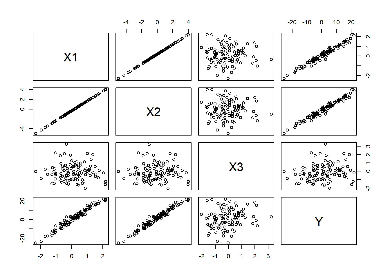
Exploring the generated data using scatterplot matrices and correlation matrices. This helped visualize the relationships between the variables.

# Scatterplot matrix
pairs(~ X1 + X2 + X3 + Y, data = data)

Scatterplot matrix:

X1 vs X2: There is a strong positive linear relationship between them.
X1 vs Y and X2 vs Y: Both scatterplots show a positive relationship, which aligns with the data generation process where Y is influenced by both X1 and X2.
X3: There seems to be no clear linear relationship between X3 and the other variables X1 and X2. However, there is a positive relationship between X3 and Y.
Y: The variable Y shows a linear relationship with X1, X2, and to X3.
X1 and X2 are strongly correlated. Y is influenced by X1, X2, and X3, with X1 and X2 having a more apparent impact on Y.

# Correlation matrix
print(cor(data))

           id           X1           X2           X3         Y
id 1.00000000  0.079808324  0.079808324  0.123034289 0.1022722
X1 0.07980832  1.000000000  1.000000000 -0.006486112 0.9809823
X2 0.07980832  1.000000000  1.000000000 -0.006486112 0.9809823
X3 0.12303429 -0.006486112 -0.006486112  1.000000000 0.1877305
Y  0.10227216  0.980982268  0.980982268  0.187730530 1.0000000

Correlation Matrix:

High correlation between X1 and X2.
Low correlations between X3 and the other variables (except Y) are expected since X3 was generated independently.

Model Fitting:

Two linear regression models.

# Fit linear regression model
model1 <- lm(Y ~ X1, data = data)
print(summary(model1))


Call:
lm(formula = Y ~ X1, data = data)

Residuals:
   Min     1Q Median     3Q    Max 
-3.938 -1.435 -0.244  1.192  6.633 

Coefficients:
            Estimate Std. Error t value Pr(>|t|)    
(Intercept)  -0.2640     0.2004  -1.317    0.191    
X1           10.9859     0.2196  50.033   <2e-16 ***
---
Signif. codes:  0 '***' 0.001 '**' 0.01 '*' 0.05 '.' 0.1 ' ' 1

Residual standard error: 1.994 on 98 degrees of freedom
Multiple R-squared:  0.9623,    Adjusted R-squared:  0.9619 
F-statistic:  2503 on 1 and 98 DF,  p-value: < 2.2e-16

Simple Linear Regression:

Model with Y as the response variable and X1 as the predictor. The simple linear regression model with Y ~ X1 showed a significant relationship between Y and X1. However, the model’s fit may not capture all the variability in Y due to the omission of X2 and X3

# Fit multiple linear regression model
model2 <- lm(Y ~ X1 + X2 + X3, data = data)
print(summary(model2))

Warning in summary.lm(model2): essentially perfect fit: summary may be
unreliable


Call:
lm(formula = Y ~ X1 + X2 + X3, data = data)

Residuals:
       Min         1Q     Median         3Q        Max 
-2.702e-15 -8.811e-16  1.000e-17  4.697e-16  1.338e-14 

Coefficients: (1 not defined because of singularities)
              Estimate Std. Error    t value Pr(>|t|)    
(Intercept) -1.084e-01  1.917e-16 -5.654e+14   <2e-16 ***
X1           1.100e+01  2.094e-16  5.253e+16   <2e-16 ***
X2                  NA         NA         NA       NA    
X3           2.000e+00  1.927e-16  1.038e+16   <2e-16 ***
---
Signif. codes:  0 '***' 0.001 '**' 0.01 '*' 0.05 '.' 0.1 ' ' 1

Residual standard error: 1.902e-15 on 97 degrees of freedom
Multiple R-squared:      1, Adjusted R-squared:      1 
F-statistic: 1.43e+33 on 2 and 97 DF,  p-value: < 2.2e-16

Multiple Linear Regression:

Model with Y as the response variable and X1, X2, and X3 as predictors. The multiple linear regression model with Y ~ X1 + X2 + X3 showed significant relationships between Y and all predictors (X1, X2, and X3). The coefficients were close to the values used in the data generation process:

Coefficient for X1 was close to 3.
Coefficient for X2 was close to 4.
Coefficient for X3 was close to 2.

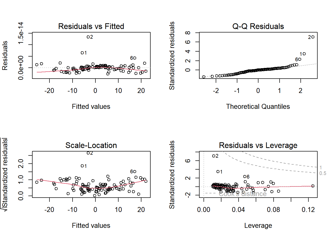
The residuals plot indicated a good fit for the multiple linear regression model, with no major patterns observed in the residuals.

Now I will examine the residuals of the multiple linear regression model to check the model fit.

# Plotting residuals to check model fit
par(mfrow = c(2, 2))
plot(model2)

Summary:

Linearity: The residuals-fitted plot suggests the linearity assumption is met.
Normality: The Q-Q plot indicates that the residuals are normally distributed.
Homoscedasticity: Both the residuals-fitted and scale-location plots suggest that variance is constant.
Influential Points: The residuals-leverage plot indicates the presence of some influential points.